Completion requirements:
- View
Learning to Represent Data
Neural networks can help us isolate some abstract attributes in data and learn representations that are suitable for solving problems.
In the examples we have used so far, we have most often relied on the existence of some set of attributes in the data set. Indeed , a large number of domains generate data that is of this form, with attributes in columns and instances in individual rows. As we saw in the introductory part of the data preparation story, even when we have these attributes, it's not the most intuitive to decide which attributes to choose to create a model. This put us in a position to try different combinations or devise techniques that can help us in the selection of attributes. Due to the complexity of the functions they model, neural networks boast the ability to learn to filter and group the attributes that matter.
This property of neural networks is especially important when working with non-tabular data - we have raised the question many times how to represent, for example, images, text data or audio recordings. Although we have knowledge of these formats, it is difficult for us to describe exactly what they contain in a concise and usable way. This, among other things, has motivated us to apply the data-driven programming paradigm. Neural networks can (and we will soon see) learn some abstract attributes from data in their source form that are useful for successfully solving problems.
Below , we will introduce convolutional neural networks that are used primarily in working with images and video and to learn visual attributes of input, and then recurrent neural networks and transformers, types of neural networks that are used to learn the attributes of sequential data such as text or sound.
Convolutional Neural Networks
Convolutional neural networks are a type of neural network that is primarily used in the field of computer vision to work with images and video content.
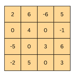
Black and white images are represented by pixel matrices. The number of types of this matrix corresponds to the height of the image, while the number of columns of this matrix corresponds to its width. The individual pixel values are numbers ranging from 0 to 255, where 0 is black and 255 is white. All the values in between represent some shade of gray. Can you guess what's behind the image that is represented by the pixel matrix below? If you step back far enough and draw contours along the darker shades, you might be able to guess what's in the picture. It helps that in the machine learning community, images of cats are a fairly common choice.
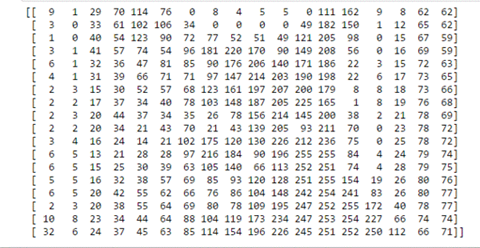
You can also check the next block and see what the picture is.
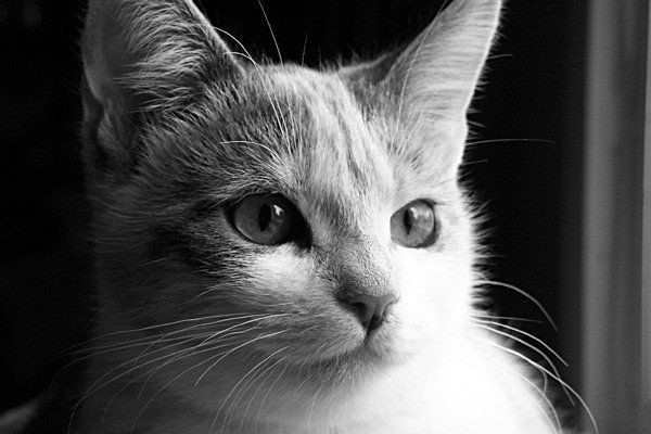
Just as it is difficult for us humans to understand what is in an image represented by a group of numbers, so it is with convolutional neural networks. They begin their analysis of the image by first recognizing some simple elements such as horizontal and vertical lines, and then combining them further and adding complexity until they arrive at some complex descriptions of the image that can help them solve the task at hand. Now the natural question is how start from simple contours and build on them to obtain more complex structures. The answer will be given by the convolutional operator .
The easiest way to introduce the convolution operator is through illustrations. Let's imagine that we have a matrix of 6x6 pixels at the input that represents the image, and a small matrix, the so-called filter, with dimensions of 3x3 pixels. Let these be the matrices shown in the image below. We start applying the convolution operator over the image (we will mark it with ✷ ) by overlapping the part of the image in the upper left corner with the filter, then multiply the individual values and write the sum of the values into a new matrix . This matrix will be the result of the application of the convolutional operator.
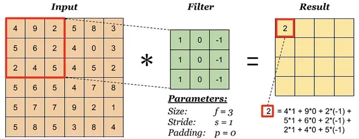
Convolution - Step 1
We will continue to apply the convolution operator: we will overlap the filter with the part of the image located in the upper left corner, but so that it is now shifted one pixel from the left edge, i.e. compared to the previous position. Again, we will multiply the individual values, add them together, and write them into the resulting matrix.
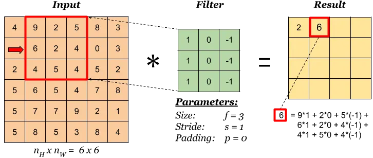
Convolution - Step 2
The filter can be moved one position to the right all the way to the edge. Then we need to lower it one position down and put it back right next to the edge. Then we can continue the process until we reach the lower right corner. As a result of this operation, we will get a matrix of dimensions of 4x4 pixels, the values of which are shown in the image below (be sure to make sure!).
Convolution - the result
How much the filter will be moved in each iteration is defined by a hyperparameter called a scroll. stride). In our case, the offset had a value of 1 because we moved the filter one position to the right, that is, when it should have been one position down. In order to be able to influence the dimensions of the resulting matrix when applying the convolutional operation (usually we want to preserve the dimensions that correspond to the input matrix), we can add a frame around the starting image. It is usually a block of zeros or ones or numbers whose values correspond to the values of the nearest pixel in the image. It's called an extension. padding ) and its width are always emphasized when applying the convolutional operation. It is especially important to us if the characteristics we want our model to learn are close to the edge of the image.
The animation below illustrates the entire process of applying filters to the image, i.e. On top of her matrix. As you can see, a size 1 offset and a size 0 extension were used.

Animation of the convolutional operation
If we apply the filter from the previous example using the convolution operation on the initial image of the kitty, we get the image below. You can see that all the vertical lines that appear in the picture are highlighted.
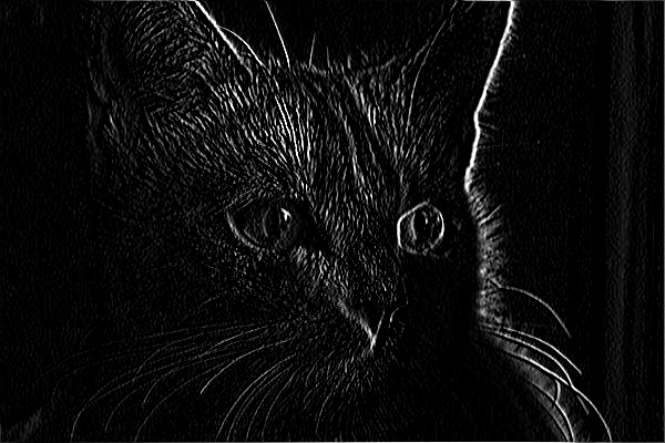
Vertical Edge Extraction
Are you surprised that the top filter detected vertical edges?
Here's an explanation.
Look at the picture from left to right. The first time you move from the light part of the picture to the dark part of the picture, you actually see a vertical edge. Let's now apply a filter from left to right with a convolutional operation. The highest result of an iteration of the convolution will be when the right side of our filter (the column numbered -1) is positioned exactly on the vertical edge. Since the edge is dark, the values that correspond to that color are small because the black color is represented by zero. The values to the left of the edge are light, so the numbers that correspond to those colors are larger (the value for white is 255). When the small values corresponding to the black color of the edges are multiplied by -1, i.e. with the right part of the filter, and the large values, which correspond to the light colors to the left of the edge, are multiplied by 0 and 1, i.e. The result is a higher value than if the filter were found anywhere else where there is no filter.
Look at the picture from left to right. The first time you move from the light part of the picture to the dark part of the picture, you actually see a vertical edge. Let's now apply a filter from left to right with a convolutional operation. The highest result of an iteration of the convolution will be when the right side of our filter (the column numbered -1) is positioned exactly on the vertical edge. Since the edge is dark, the values that correspond to that color are small because the black color is represented by zero. The values to the left of the edge are light, so the numbers that correspond to those colors are larger (the value for white is 255). When the small values corresponding to the black color of the edges are multiplied by -1, i.e. with the right part of the filter, and the large values, which correspond to the light colors to the left of the edge, are multiplied by 0 and 1, i.e. The result is a higher value than if the filter were found anywhere else where there is no filter.
How would you separate the horizontal edges in the picture? Which filter would you use?
All you have to do is rotate the filter that separates the vertical edges! Does that make sense to you?
Now that we know how to separate vertical and horizontal edges, we can combine in a variety of ways to single out lines that are not just horizontal and vertical. By further combining these results, we can even extract spherical contours. This is what we meant when we said that we start with clear, easy-to-learn characteristics, and then build step by step on the complexity of the characteristics we can learn.
The layers of a neural network characterized by the application of the convolutional operator are called convolutional layers. While the pioneers in the field of computer vision created filters manually, the goal of training convolutional neural networks is to learn for themselves the values that figure in them.
In the image below, you can see the representations of the learned filters on the layers of a convolutional neural network that recognizes faces. On the lowest layer, these are some horizontal, vertical and diagonal lines, on the second layer these are already outlines that correspond to parts of the face such as the nose, eyes and mouth, while on the third layer these are filters that correspond to the contours of the face.
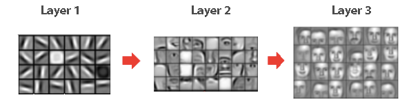
Classification process of passing through successive layers of the image
In addition to the convolutional operation, convolutional networks are also characterized by the pooling. As the name suggests, the goal of this operation is to pool, i.e. consolidate the entrances. In the image below, you can see two types of pooling operators: the one that uses the maximum and the one that uses the average to pool the information. Just like the convolutional operator, this operator is applied to blocks of input by noticing the block and performing the necessary calculation on it. The value obtained in this way is entered into a new matrix. In the figure, both operators are applied to 2x2 blocks. Intuitively speaking, we emphasize the most dominant part with maxima, while by calculating the average, we take into account the contribution of all parts.
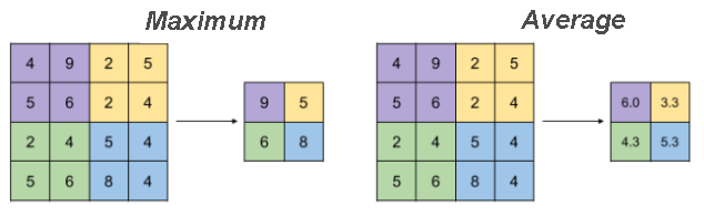
By applying the pooling operation, we get the ability to reduce the dimension of the input, but at the same time retain some of the information that is contained. In the image you can see that by applying the pooling operator, we have reduced the matrix from 4x4 to 2x2. Why do we need dimension reduction? As a result, the network needs to give us a specific answer, let's say whether there is a cat in the picture or not, for which we need a small number of neurons.
The layers of a neural network that are characterized by the application of the pooling operator are called pooling layers. There are no additional parameters in them that the network needs to learn, but, as we have seen, they help us control the dimensions of the matrices we work with.
Now that we know what the building blocks of a convolutional neural network are, let's see how we can connect them and get a functional model that can help us solve the classification task. Let's imagine that we need to solve a multi-class classification task in which for each image of a cartoon character we need to determine whether it is Tweety, Goofy or Dacia Duck. Let's look at an illustration of the architecture of a deep convolutional neural network that we have chosen to solve this task and discuss what is the motivation for its creation.
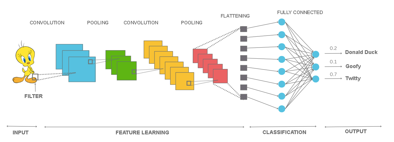
At the beginning of the network there is an input layer that contains pixels of the image. This is followed by a convolutional layer (a blue block). The goal of this layer is to use the convolution operator to extract the first set of abstract attributes. After that, we place an pooling layer (green block), followed by another convolutive layer (orange block) and an pooling layer (red block). In practice, the convolution and pooling layers are combined and often located next to each other because the pooling layers are further pooled, i.e. summarizes what the convolutional layers have learned. The second convolutional layer allows us to apply a second convolutional operator to attributes already extracted by the first convolutional layer and form more complex image attributes. This block of layers is followed by a layer (gray block) that has the task of "correcting" the matrix (or, more precisely, the tensor) that we have received up to that point and repackaging its values so that they are all next to each other in one array. Layers for this purpose are called straightening layers. flattening layers ). After correction, we can further build on a fully connected neural network. This network will now have abstract attributes as inputs that a combination of convolutional layers and pooling layers learns for it. In addition to the corrected input layer, we also see a hidden layer in the image as well as an output layer in which there are exactly three neurons - one for each of the cartoon characters. The output values of these neurons correspond to the probability that the input image belongs to the class they represent. For the image of Twitter that we have at the input, we can notice that the output value of the third neuron, which corresponds exactly to that class, is the largest and is 0.7.
Now we can also see what the architecture of the VGGNet network looks like, a popular convolutional network that is actively used in practice.
VGGNet is a deep convolutional neural network developed by the Oxford team Visual Geometry Group (hence the name VGGNet ). At the prestigious Large Scale Visual Recognition Challenge , held in 2014, this network proved to be the best in solving the problem of localization of objects in an image and as the second in a row in the problem of classifying objects from an image. Over 1.2 million images were used for the classification task of the ImageNet set that we have come to know and the classification into a possible 1000 classes. To train this network it took between 15 and 20 days using 4 graphics cards (the best at the time) NVIDIA Titan Black . Before it, the best in these tasks was the AlexNet network , which is notable for introducing the practice of using graphics cards to train neural networks and allow the further development of deep learning.
The architecture of the VGG-16 network, a version of the network with 16 layers, is shown in the image below. As we can see, a color image measuring 244x244 pixels is expected at the input, and the network combines convolutional layers and pooling layers (with maximum) and ends up with a fully connected neural network with 1000 neurons at the output, where each neuron corresponds to one particular class of the ImageNet set. The network itself has 138 million parameters and requires about 500 MB of memory to store them.
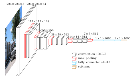
VGG-16 Network Display
Increasing the number of layers of the convolutional part of the network usually gives better results in practice. However, the number of layers cannot increase indefinitely. Not only because of the limitations of resources, time, and cost, but also because of the mathematical properties of deep neural networks, which further make it difficult to apply the backward propagation algorithm and train the network itself.
If you are interested in this mathematical problem, you can try to read more about disappearing and exploding gradients, especially in the part of convolutional networks and residual connections.
Before we get into the task of working with convolutional neural networks, let's take a look at the issue of working with color images. We haven't mentioned them so far.
When we need to present a color image, one that uses the RGB color format and displays all colors as combinations of red, green and blue, we use three matrices. One matrix is provided for each of the colors. The number of matrices we use to display images is called channels . Thus, black and white images have only one channel, while color images have three channels.
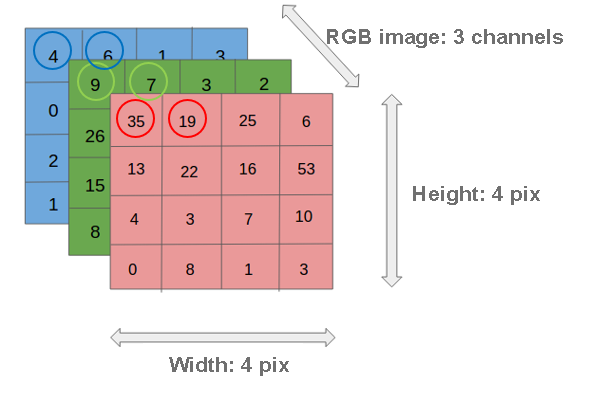
Display of images that use the RGB color format
The presence of colors affects the performance of the convolutional operation by adjusting the number of channels of the filter to the number of channels of the image to which we are applying it. Next, you need to pair each of the filter channels with the image channel (red with red, blue with blue, and green with green) and perform the convolutional operation as if you were working with a single channel. Then we need to add the matrices that we get in this way and declare the resulting matrix as the final result. In the image below, we can see two filters in a convolutional layer that are applied over the color input image. As a result of applying each of these filters, we will get separate matrices that, when "merged", represent the final result of the convolutional layer. In practice, multiple filters are usually placed at the level of one convolutional layer, so tensors are obtained as results. Convolutional operations are then applied to these tensors in the same way - only care is taken to ensure that the number of filter channels corresponds to the dimension of the tensor (let's say, for the next application in the example we considered, this would be the number 2) and that the corresponding input channel is paired with the corresponding filter channel.
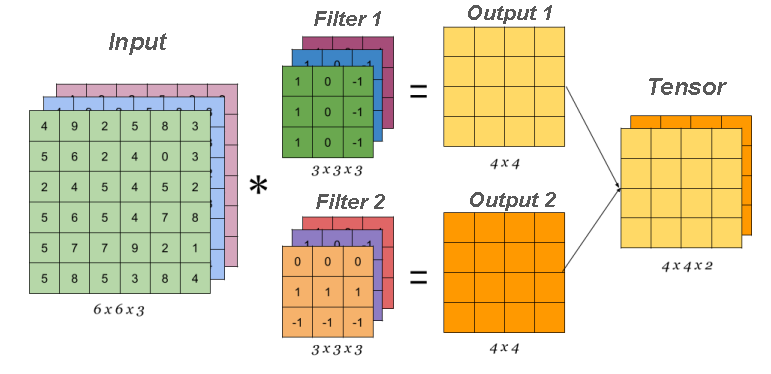
Applying the Convolutional Operator to Multi-Channel Inputs
As for the pooling operation, it is applied over each channel of the input image. For example, if the input image has 3 channels, the pooling operation will be applied to each channel separately. This also means that the pooling operation preserves the number of channels at the time of deployment. In the picture below you can see an illustration of this process.
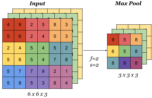
Applying pooling Operators to Multi-Channel Inputs
This section is paired with the Jupyter Notebook 11-VGG-16_network_and_classification.ipynb. To follow the content further, click on the link and then click  on the button to open the content in Google Colab . If you are viewing the notebooks on your local machine, find the notebook with the same name among the contents and run it. For more detailed instructions, see the Hands-on Zone section and the Jupyter Notebooks lesson for practice .
Now let's try out how the VGG-16 convolutional network really works! Don't forget to follow the notebook with the code while reading the lesson.
Once trained, a neural network model can be shared with the community by dividing the parameters that figure in it. In this example, we will use the model that is available in the Keras library. The Keras library is an open source library widely used in the machine learning community. In order to take advantage of the VGG-16 network model , we need to execute the following two commands:
from tensorflow.keras.applications import VGG16
model = VGG16(weights='imagenet')
We can read the information about the model we have loaded using the model.summary() function. Its result is a description of the network layers followed by information about the input sizes that these layers expect. Now you can execute the command:
model.summary()Don't be confused if you don't understand all the details that are displayed after executing this command. It's important to know that the input is expected to be an image with dimensions of 224x224 pixels in color (that's why 224, 224, 3 is listed next to the input layer) and that you have one of 1000 classes at the output. You can also compare the print with the image of the VGG-16 we discussed to reveal more information.
It is important to emphasize that we will not train the VGG-16 network - we will use only a trained model. Therefore, we must not change the parameters of the model during operation - each has its own contribution. The total number of model parameters that we can read in the network summary is just over 138 million.
The idea is that the image on which we are going to test the model will be an arbitrary image from the web. To do this, we will use a number of standard Python libraries. To default the URL function ucitaj_sliku will help us drag the image we want.
def load_image(url_path):
	response = request.urlopen(url_path, context=ssl_context).read()
	return Image.open(BytesIO(response))
For testing, we have chosen a picture of a Golden Retriever from address https://unsplash.com/photos/x5oPmHmY3kQ , which can be used freely. You can choose the image you want! It is important to keep in mind that the class of the object in the picture must be known to the model. Since the VGG-16 model has been trained on over 1.2 million images, it knows a lot of classes, as many as 1000 different ones. The Golden Retriever is one of them. If we give the model a picture with an object that it does not know, It will give us predictions of the classes whose images most closely resemble ours. We'll see in the end which classes resemble the Golden Retriever.
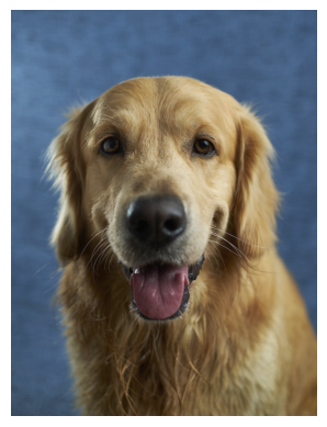
The hero of the story of the VGG-16 model
Since the image that needs to be forwarded to the model needs to be specially prepared, we will do the following:
set its dimensions to 224x224 and tell it to use three RGB color channels:
test_image = test_image.resize((224, 224))
test_image = test_image.convert('RGB')
Transform the image into a suitable matrix format:
matrix_form_test_image = image.img_to_array(test_image)make a package that contains our picture:
batch = np.expand_dims(matrix_form_test_image, axis=0)Perform numerical image preprocessing in the form of normalization:
test_image_batch = preprocess_input(batch)Only in this way can we pass on the model for classification. The function that will help us is (expectedly) called predict.
model_predictions = model.predict(test_image_batch)The variable predikcije_modela in which we store the predictions of the model is an array of length 1000 and contains the probabilities of belonging to each of the 1000 classes that the model recognizes. To extract the class to which our image belongs, we can use the decode_predictions function, which will return the probabilities and names for the 5 most probable classes. This will give us an insight into how secure the model is when classifying. After executing the next command, we will get information about the most likely classes.
most_likely_classes = decode_predictions(model_predictions)[0]When we graphically represent these predictions with the code listed below, we get a graph with bars that allows us to more easily analyze the results.
class_names = [item[1] for item in most_likely_classes]
class_probabilities = [item[2] for item in most_likely_classes]
plt.figure(figsize=(10, 4))
plt.bar(class_names, class_probabilities, color=['teal', 'yellow', 'green', 'blue', 'orange'])
plt.title('Top 5 Most Likely Classes')
plt.ylabel('Probability')
plt.show()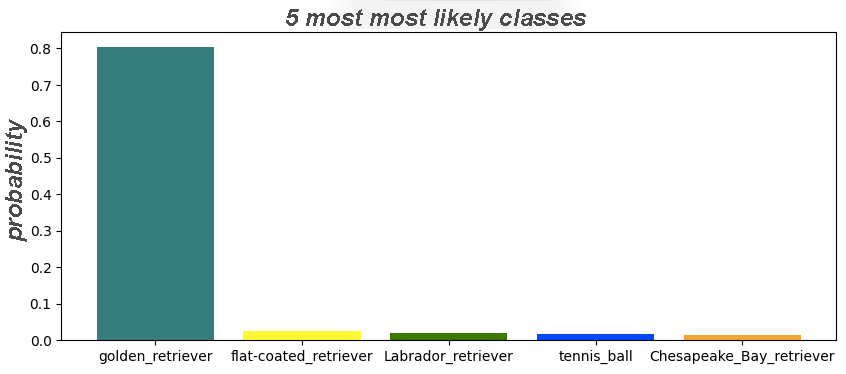
As we can see, the model predicted with great certainty (probability is 0.804) that the image we chose was that of a golden retriever. Some of the other classes that the model has taken into account are some other types of retrievers. Oddly enough, a tennis ball also appeared in the list of results. Probably because in the training set there are also images in which retrievers run after tennis balls. This behavior of the model should be further investigated in practice.
Last modified: Thursday, 26 June 2025, 11:19 PM