3.8 K-Nearest Neighbor (kNN) Algorithm

Let our training set consist of pairs of numbers \((x_1,x_2)(x_1,x_2)\) and the corresponding class names. Pairs can be represented as points in the plane, where the first coordinate \(x_1\) denotes the value on the x-axis and the second coordinate \(x_2\) denotes the value on the y-axis. In practice, the values of \(x_1\) and \(x_2\) are always associated with some specific attributes, for example, temperature and humidity, but now we can think of them as some general values. Each pair of numbers belongs to one of two classes: red triangles or blue squares. Since there are only two classes, you can assume that it is a binary classification. Now imagine that the green circle represents a new instance, a new pair of numbers, for which we need to determine which class it belongs to: whether it is a red triangle or a blue square.

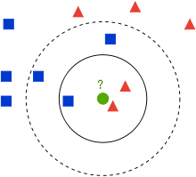
Training Kit

The k-nearest neighbor algorithm is a classification algorithm that says that we first fix the number of neighbors (surrounding instances) k to a specific value and then determine how many of the k-closest neighbors there are red and blue: the red neighbor is an instance belonging to the red class, and the blue neighbor is an instance belonging to the blue class. For example, if we fix the number k to 3, the three closest neighbors of the green circle are inside a solid circle. There are two red triangles and one blue square.

Further, the k-nearest neighbor algorithm says that the new instance, a new pair of dots is added to the class of the more numerous neighbor: if the red neighbors are more numerous, we say that the new instance belongs to the red class, and, similarly, if the blue neighbors are more numerous, we say that the new instance belongs to the blue class. You can also think of this as the saying "who you are with, that's who you are" in the world of machine learning.

In our example, when the value of k is fixed at 3, we conclude that we should associate the green circle with the red class because we have two red neighbors and one blue neighbor.

Let's see what happens if we fix the number k at 5. In the figure this neighborhood is shown by a dashed circle. Since there are now three blue squares and two red triangles, the conclusion would be that the green circle should be joined to the blue class.

 This section is paired with Exercise 8 and Jupyter Notebook 08-k-nearest_neighbors.ipynb. To follow the content further, click on the link and then on the button to open the content in Google Collab. If you are viewing the notebooks on your local machine, find the notebook with the same name among the contents and run it. For more detailed instructions, see the Hands-on Zone section and the   Jupyter Notebook Practice Lesson.

The accompanying material contains the aforementioned set of points and an application in which you can examine what will happen if you choose a different value of the number k. Since the algorithm needs to decide which neighbors there are more, it is wise to choose odd values of the number k.

Note that in addition to the number of neighbors k, the result of the algorithm also depends on how we measure the distances to the neighbors! To find the nearest neighbors, we need to somehow measure the distance to them.

Until now, we have encountered a distance called the Euclidean distance. The Euclidean distance between the points \(A\) and \(B\) is calculated as the length of the lengths connecting the points \(A\) and \(B\). For example, for the points \(A =(0,0)\) and \(B =(3,4)\), the Euclidean distance is calculated as \(\sqrt{(3 − 0)^2 +(4 − 0)^2} = 5\)

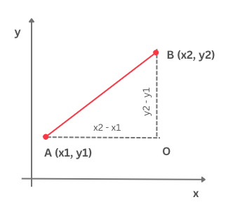
Euclidean distance

There are many other distances as well. For example, you may be intrigued by the Manhattan distance. Unlike the Euclidean distance, which calculates the "hypotenuse" of a triangle defined by the points \(A\) and \(B\) and \(O\) (if we follow the previous figure), the Manhattan distance calculates the sum of the "legs" of this triangle. For points \(A\) and \(B\), the value of the Manhattan distance would be \(| 3 − 0 | + | 4 − 0 | = 7\).

Which distance we choose depends on the nature of the task and the meaning that the attributes we are working with have. In general, we can try more distances and choose the one for which we get the best results. We will talk about this later. It is important to note that a function must satisfy certain mathematical properties in order to be declared a distance, so not every function can be helpful.

 Just like other machine learning algorithms, the x-nearest neighbor algorithm is trained over the training set. It is interesting to note that the learning phase in this algorithm is actually reduced to storing the dataset only. In other algorithms, such as linear regression or logistic regression, we have seen that in this phase, the values of some parameters that appear in the model are calculated by looking for the minimum error function. The x-nearest neighbor algorithm is not like that. The mapping we learn It's not about a specific function, it's about the data itself and the steps that need to be taken. That is why it is common to call models that have this property nonparametric models. 

The k-nearest neighbor algorithm performs all the work during the application, i.e. Decide which class the new instance belongs to. When we need to classify a new instance, we first calculate the distance of the new instance from all instances in the training dataset. Next, we sort these distances from smallest to largest. We keep the first k distances (because they are the distances to k closest neighbors) and choose instances from the training set to which they refer. We continue to monitor what is happening in the space of their landmarks and look for the most numerous landmarks, i.e. the largest class. As we saw in the introductory example, the new instance should be associated with the class that is the most numerous.

This algorithm is easy to implement, so let's roll up our sleeves and get started!

Let's imagine that we are working with a set of data that we have used so far and that each instance has a form \((x1, x2, mark)\) where the \(mark\) is the value 0 for red or 1 for blue.

To measure the distance between instances, we will use the euklidsko_rastojanje function, which is defined by the following block of code:

def euclidean_distance(instance1, instance2):
  return np.sqrt((instance1[0]-instance2[0])**2 + (instance1[1]-instance2[1])**2)

The x-nearest neighbor algorithm itself is represented by the following block of code:

def kNN(k, instances, new_instance, classes={0: 'red', 1: 'blue'}):

  # first, calculate the distances between the new instance and all instances in the dataset
  distances = [euclidean_distance(instance, new_instance) for instance in instances]

  # then sort the distances, extract the k smallest ones and the corresponding instances
  # declare them as neighbors
  neighbors = np.argsort(distances)[0:k]

  # then read the labels of the neighbors and count them
  neighbor_labels = [instances[neighbor][2] for neighbor in neighbors]
  label_counts = np.bincount(neighbor_labels)

  # the label of the new instance will be the label of the most frequent neighbor
  label = np.argmax(label_counts)

  return classes[label]

In it, as we have discussed, we carry out the following steps:

1. We calculate the distance from the new instance to all instances in the data set.
2. And then we put them in the middle of the night, and then we put them in the dark.
3. And we are the ones who have the right to be the neighbors.
4. In the set of isolated neighbors, we count the most numerous,
5. We conclude that the new instance belongs to the class of the most numerous neighbor.

We still have to learn how to choose the best value of the number k. We will talk about this in the next lesson.

Show answer

Show answer