3.6 Logistic regression

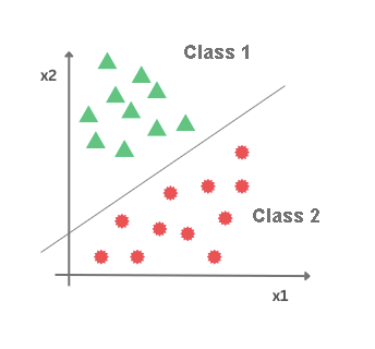
Let's imagine that we have a data set with two attributes, \(X_1\) and \(X_2\), and that the instances of this set are shown as in the figure below. Along the x-axis, the \(X_1\) attribute is represented, along the y-axis, the \(X_2\) attribute, and the color of the dots indicates the class to which each of these instances belongs. You will agree that a linear model that determines a line in a plane could help us solve the classification problem by separating the classes - one below this line and the other above. In order to be able to conclude in this way, we will benefit from the sigmoid function.

The sigmoid function is a popular function in the machine learning story. It is determined by the equation

\(σ(x)=\frac{1}{1+e^{−x}}\)

Her picture looks like the one in the picture below.

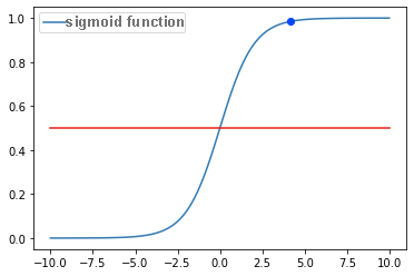
Graph of sigmoid function

We can immediately notice that this function takes a range of values from 0 to 1. The smaller the values of \(x\), the closer the value of this function is to 0 and, similarly, the larger the value of \(x\), the closer the value of the sigmoid function is 1. For \(x= 0\), the value of the sigmoid function is 0.5. If we declare this value as a threshold and introduce the rules:

1. If the value of the sigmoid function is greater than or equal to 0.5, associate x with a positive class and
2. If the value of the sigmoid function is less than the threshold of 0.5, associate x with the negative class

we will get a function suitable for the classification task.

It also seems to us that the higher the values of x, the more convincing the decision to associate x with a positive class, because we significantly exceed the threshold value. It also seems that the smaller the values of x, the more plausible the decision to join x to the negative class, because we are significantly below the threshold value. For values of x, which are around zero, these arguments are weaker. Therefore, the sigmoid function can also be associated with the interpretation of the probability of belonging to a class.

If we connect the sigmoid function and the equation of the linear model, we get the equation of the logistic regression model, which in general is

\(y=σ(X_1,X_2,...,X_n)=\frac{1}{1+e^{−(ꞵ_0+ꞵ_1X_1+ꞵ_2X_2+ꞵ_3X_3+...+ꞵ_nX_n)}}\).

The arguments \(X_1, X_2, ..., X_n\) denote attributes in the data set, while its uu values range from 0 to 1 and, as we have seen, make sense for the classification task. To this equation we can also add the following geometric interpretation: the data is classified either below or above the "line" that is determined by the linear relationship equation that we initially imagined.

Cross-entropy

The error function that characterizes logistic regression is called cross-entropy. Let's first get to know the intuition that lies behind this function, and then let's get to know its mathematical form.

 We have said that we interpret the value calculated by the logistic regression model as the probability of belonging to one of the classes, and that we are guided by the rule that if this value exceeds the threshold of 0.5, we interpret it as belonging to a positive class, and if this value is less than 0.5, we interpret it as belonging to a negative class. If the probability value is 0.5, it is interpreted as belonging to a positive class.

We calculate the error function on the training set. In it, we know for each instance what the exact characteristics are, so we can always compare them with the characteristics that he calculated, i.e. I've joined the model.

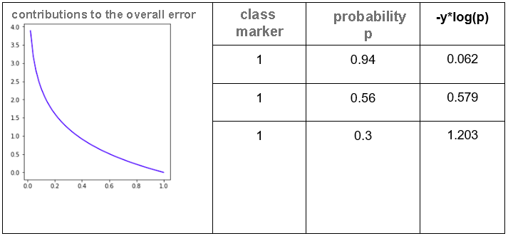
Suppose that for three instances belonging to a positive class, the logistic regression model calculated the values 0.94, 0.56, and 0.3 respectively. In the first case, the value is close to the unit, so it indicates a certain decision of the model. In the second case, this value is smaller and closer to the classification threshold, but sufficient for a good decision of the model. In the third case, the value is below the threshold and would cause the model to make an error. When designing the error function, we want to penalize the calculations of the model that for positive The value is more than 1, i.e. to make their contributions to the overall error of the model greater. One such function that satisfies the required property is \(− log(x)\), the graph of which is shown in the figure below. We need a minus sign for the error to get a positive value because the logarithm is negative for the values of the function argument that are from 0 to 1. In the graph we can also see that the values of the function are small for arguments closer to 1, i.e. That the values of the function are greater for arguments that are closer to zero. So now, in order, the contributions to the total error of the extracted instances will be \(− log(0.94)= 0.062\), \(− log(0.56)= 0.579\) and \(− log(0.3)= 1.203\) and exactly the size ratio we wanted. We can also record them in a table, the way we did and in the linear regression task. In the first column, we will place the class marker (the exact value), in the second column the probability p calculated by the model, and in the third column we will enter the value \(− log(p)\). Note that the column name says \(− y ∗ log (p)\), but since \(y = 1\), this is the same as \(− log(p)\).

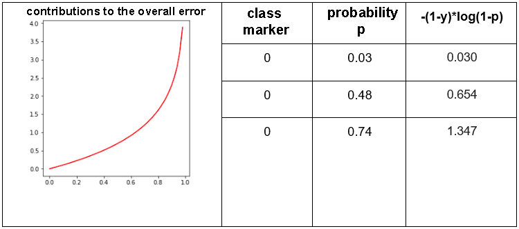
 Let us now select three instances of the negative class and discuss the expectations we have of the error function in their case. Let the probabilities, respectively, calculated by the logistic regression model be 0.03,0.48 and 0.74. Now, in the first case, the value of the model is close to zero, so it indicates a certain decision to belong to the negative class. In the second case, this value is close to the classification threshold, but it isbelow it, so again it is enough for the model to decide on a negative class. In the case of the third instance, the probability value is over the threshold, so the model will err and classify the instance as positive. What we expect from the error function for negative instances is that their share of the total error is as high as possible the farther away they are from zero. One such function that satisfies this property is − log(1 − p) and its graph is shown in the figure below. Again, we use a function with a minus sign to make the error value positive. We can now write the values of this function in a table. The first column now contains the instances with a value of 0, the second column contains the probabilities p that the model calculated, and the last column contains the values of the error functions \(− log(1 − p)\). Since \(y = 0\) for all instances, the symbol in the column name \(−(1 − y) ∗ (1 − p)\) does not change anything.

 The total value of the cross-entropy functions is obtained when the error contributions of all positive and all negative instances are added together (similar to what we did in the linear regression and mean-squared error problem). This is written in the form

\(−\sum\limits_{i = 1}^{N}(y_i⋅log(p_i)+(1−y_i)⋅log(1−p_i))\)

where the first factor sums the contributions of the errors of the positive instances, and the second factor contributes the errors of the negative instances. The value of yi is the exact characteristic of the class in the training set, and pi is the probability calculated by the logistic regression model. This error is called binary crossentropy.

 The values of unknown \(β\) parameters in the logistic regression model are found by selecting the parameter value for which the cross-error function is the smallest. The gradient descent technique can help us in this case as well.

 Now let's get to know a slightly different classification algorithm.