Completion requirements:
- View
What if your data is actually more complex than a simple straight line? Surprisingly, you can actually use a linear model to fit nonlinear data. A simple way to do this is to add powers of each feature as new features, then train a linear model on this extended set of features. This technique is called Polynomial Regression.
Polynomial Regression is a regression algorithm that models the relationship between a dependent(y) and independent variable(x) as nth degree polynomial. The Polynomial Regression equation is given below:
$$y= \beta_0+β_1x_1^1+ β_2x_1^2+ β_3x_1^3+...... β_nx_1^n$$
It is also called the special case of Multiple Linear Regression in ML. Because we add some polynomial terms to the Multiple Linear regression equation to convert it into Polynomial Regression.
It is a linear model with some modification in order to increase the accuracy.
The dataset used in Polynomial regression for training is of non-linear nature.
It makes use of a linear regression model to fit the complicated and non-linear functions and datasets.
Hence, "In Polynomial regression, the original features are converted into Polynomial features of required degree (2,3,..,n) and then modeled using a linear model."
The need of Polynomial Regression in ML can be understood in the below points:
- If we apply a linear model on a linear dataset, then it provides us a good result as we have seen in Simple Linear Regression, but if we apply the same model without any modification on a non-linear dataset, then it will produce a drastic output. Due to which loss function will increase, the error rate will be high, and accuracy will be decreased.
- So for such cases, where data points are arranged in a non-linear fashion, we need the Polynomial Regression model. We can understand it in a better way using the below comparison diagram of the linear dataset and non-linear dataset.
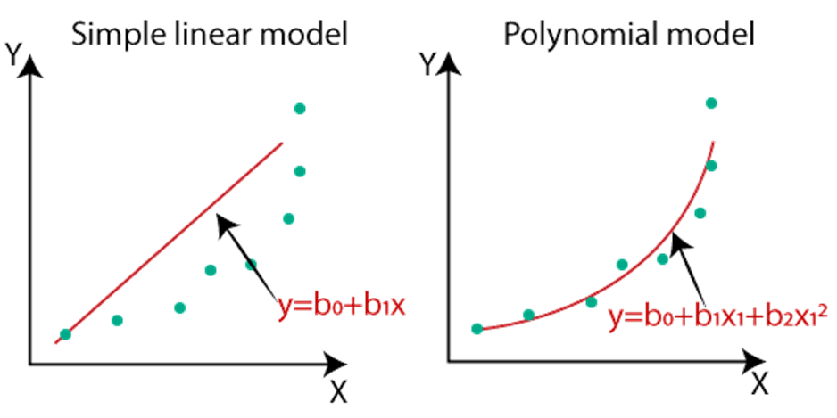
- In the above image, we have taken a dataset which is arranged non-linearly. So if we try to cover it with a linear model, then we can clearly see that it hardly covers any data point. On the other hand, a curve is suitable to cover most of the data points, which is of the Polynomial model.
- Hence, if the datasets are arranged in a non-linear fashion, then we should use the Polynomial Regression model instead of Simple Linear Regression.
| Simple Linear Regression equation |
\(y= β_0+β_1x_1\) |
| Multiple Linear Regression equation |
\(y= β_0+β_1x_1 + β_2x_2 + +...... β_nx_n\) |
| Polynomial Regression equation | \(y= β_0+β_1x_1^1 + β_2x_1^2 +...... β_nx_1^n\) |
Implementation of Polynomial Regression using Python:
Here we will implement the Polynomial Regression using Python. We will understand it by comparing Polynomial Regression model with the Simple Linear Regression model. So first, let's understand the problem for which we are going to build the model.
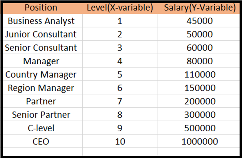
Problem Description: There is a Human Resource company, which is going to hire a new candidate. The candidate has told his previous salary 160K per annum, and the HR have to check whether he is telling the truth or bluff. So to identify this, they only have a dataset of his previous company in which the salaries of the top 10 positions are mentioned with their levels. By checking the dataset available, we have found that there is a non-linear relationship between the Position levels and the salaries. Our goal is to build a Bluffing detector regression model, so HR can hire an honest candidate. Below are the steps to build such a model.
Steps for Polynomial Regression:
The main steps involved in Polynomial Regression are given below:
- Data Pre-processing
- Build a Linear Regression model and fit it to the dataset
- Build a Polynomial Regression model and fit it to the dataset
- Visualize the result for Linear Regression and Polynomial Regression model.
- Predicting the output.
Data Pre-processing Step:
The data pre-processing step will remain the same as in previous regression models, except for some changes. In the Polynomial Regression model, we will not use feature scaling, and also we will not split our dataset into training and test set. It has two reasons:
- The dataset contains very less information which is not suitable to divide it into a test and training set, else our model will not be able to find the correlations between the salaries and levels.
- In this model, we want very accurate predictions for salary, so the model should have enough information.
The code for pre-processing step is given below:
# importing libraries
import numpy as nm
import matplotlib.pyplot as mtp
import pandas as pd

#importing datasets
data_set= pd.read_csv('Position_Salaries.csv')

#Extracting Independent and dependent Variable
x= data_set.iloc[:, 1:2].values
y= data_set.iloc[:, 2].values
Building the Linear regression model:
Now, we will build and fit the Linear regression model to the dataset. In building polynomial regression, we will take the Linear regression model as reference and compare both the results. The code is given below:
#Fitting the Linear Regression to the dataset
from sklearn.linear_model import LinearRegression
lin_regs= LinearRegression()
lin_regs.fit(x,y)
In the above code, we have created the Simple Linear model using lin_regs object of LinearRegression class and fitted it to the dataset variables (x and y).
Output:
Out[5]: LinearRegression(copy_X=True, fit_intercept=True, n_jobs=None, normalize=False)
Building the Polynomial regression model:
Now we will build the Polynomial Regression model, but it will be a little different from the Simple Linear model. Because here we will use PolynomialFeatures class of preprocessing library. We are using this class to add some extra features to our dataset.
#Fitting the Polynomial regression to the dataset
from sklearn.preprocessing import PolynomialFeatures
poly_regs= PolynomialFeatures(degree= 2)
x_poly= poly_regs.fit_transform(x)
lin_reg_2 =LinearRegression()
lin_reg_2.fit(x_poly, y)
In the above lines of code, we have used poly_regs.fit_transform(x), because first we are converting our feature matrix into polynomial feature matrix, and then fitting it to the Polynomial regression model. The parameter value(degree= 2) depends on our choice. We can choose it according to our Polynomial features.
After executing the code, we will get another matrix x_poly, which can be seen under the variable explorer option:
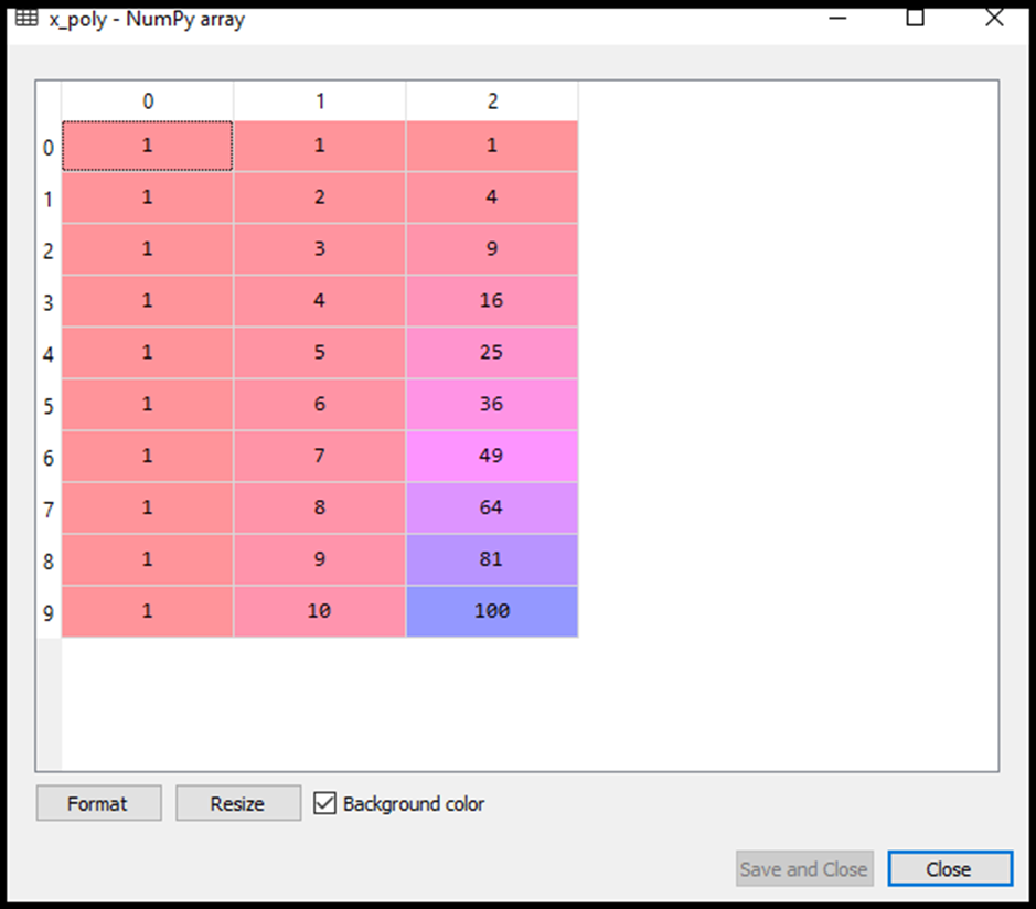
Next, we have used another LinearRegression object, namely lin_reg_2, to fit our x_poly vector to the linear model.
Output:
Out[11]: LinearRegression(copy_X=True, fit_intercept=True, n_jobs=None, normalize=False)
Visualizing the result for Linear regression:
Now we will visualize the result for Linear regression model as we did in Simple Linear Regression. Below is the code for it:
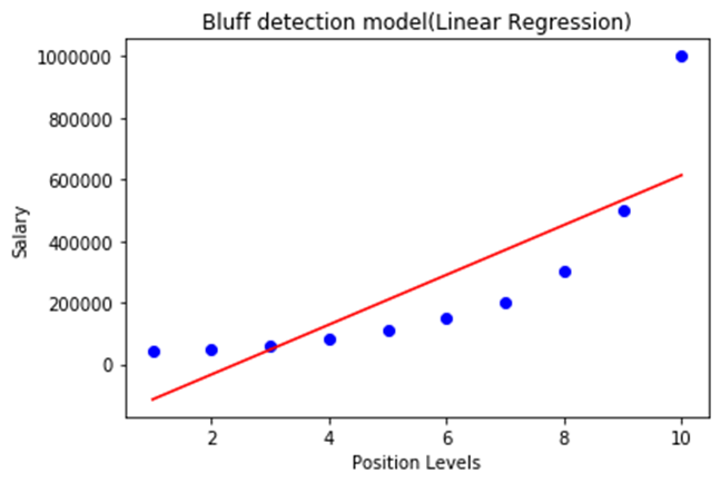
In the above output image, we can clearly see that the regression line is so far from the datasets. Predictions are in a red straight line, and blue points are actual values. If we consider this output to predict the value of CEO, it will give a salary of approx. 600000$, which is far away from the real value.
So we need a curved model to fit the dataset other than a straight line.
Visualizing the result for Polynomial Regression
Here we will visualize the result of Polynomial regression model, code for which is little different from the above model.
Code for this is given below:
#Visulaizing the result for Polynomial Regression
mtp.scatter(x,y,color="blue")
mtp.plot(x, lin_reg_2.predict(poly_regs.fit_transform(x)), color="red")
mtp.title("Bluff detection model(Polynomial Regression)")
mtp.xlabel("Position Levels")
mtp.ylabel("Salary")
mtp.show()
In the above code, we have taken lin_reg_2.predict(poly_regs.fit_transform(x), instead of x_poly, because we want a Linear regressor object to predict the polynomial features matrix.
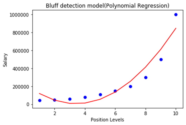
As we can see in the above output image, the predictions are close to the real values. The above plot will vary as we will change the degree.
For degree= 3:
If we change the degree=3, then we will give a more accurate plot, as shown in the below image.
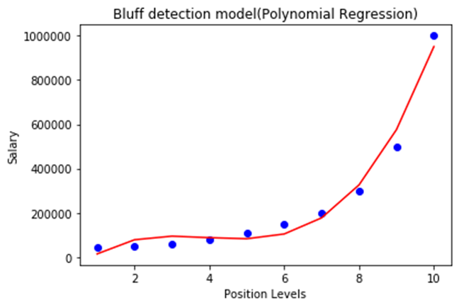
SO as we can see here in the above output image, the predicted salary for level 6.5 is near to 170K$-190k$, which seems that future employee is saying the truth about his salary.
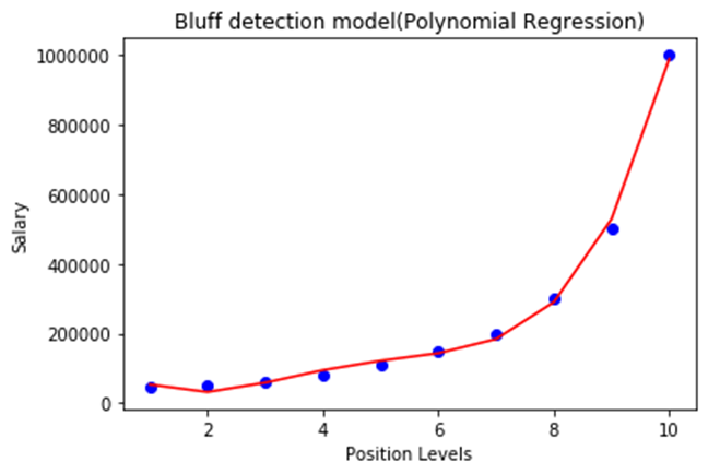
Degree= 4: Let's again change the degree to 4, and now will get the most accurate plot. Hence we can get more accurate results by increasing the degree of Polynomial.
Predicting the final result with the Linear Regression model:
Now, we will predict the final output using the Linear regression model to see whether an employee is saying truth or bluff. So, for this, we will use the predict() method and will pass the value 6.5. Below is the code for it:
Last modified: Sunday, 22 June 2025, 10:28 AM