4.1 Neural networks

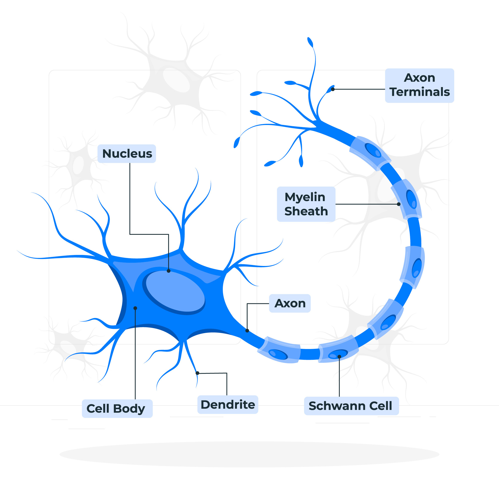
You know from biology classes that the cell is the basic unit of structure and function of all living things. From the point of view of artificial intelligence and learning, the most interesting are brain cells. These are called neurons. Neurons consist of a body with a nucleus and longer and shorter extensions, called axons and dendrites. Extensions allow neurons to connect with other neurons. These connection points of neurons are called synapses. They allow the signals, i.e. Electrical impulses generated by one neuron are transmitted to another neuron. Interestingly, one neuron can be connected to millions of other neurons. This means that it receives and processes signals coming from a multitude of other neurons and, based on its internal mechanisms, fine-tunes the signal that it sends to other neurons. It is common for this condition to be called the state of neuronal activation. It lasts only a fraction of a second, but it allows subtle calculations to be made and generates a signal that is transmitted throughout the nervous system.

The neuron we encounter in artificial intelligence is a mathematical abstraction of the brain's neurons. It is described as a function of multiple variables \(f(x_1,x_2,...,x_n)\), where each of the variables \(x_1, x_2, ..., x_n\) corresponds to a single signal that reaches the neuron. Since not all signals are equally important for neuronal activity, they are joined by weights \(w_1, w_2, ..., w_n\) that should indicate their importance. Higher values of these numbers indicate that the signal is more important, and lower values indicate that the signal is less important. Thus, the total stimulation of neurons corresponds to the weight sum \(w_1x_1 + w_2x_2 +...+ w_nx_n\). In order to influence additional neuronal behaviors, one free term b is added to this sum, so that the total stimulation of the neuron is actually \(w_1x_1 + w_2x_2 +...+ w_nx_n + b\). This is then passed on to the so-called activation function φ, which has the task of calculating the output of the neuron. Depending on the choice of activation function, the output values that are obtained will also depend. If we now write everything down systematically, we get that for the received signals \(x_1, x_2, ..., x_n\), the output of the neuron is \(y = φ(w_1x_1 + w_2x_2 +...+ w_nx_n + b\). You can also follow the procedure we have described in the illustration below.

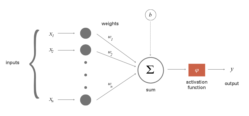
Mathematical abstraction of neurons

When neurons are connected to each other, we have a neural network. A neural network usually consists of layers, especially associated groups of neurons.

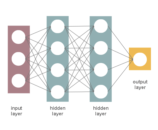
Neural network layers

The input layer is a layer that is located at the input of a neural network. The input signals \(x1, x2, ..., xn\) of this layer are related to the values of the attributes we have in the data set, and thus we approach the practical application of neural networks. For example, if we have a data set containing three attributes, temperature, humidity and atmospheric pressure, the input layer will have three neurons: the first will correspond to the first attribute, temperature, the second will correspond to the second attribute, humidity, and the third neuron to the third attribute, i.e. the atmospheric pressure. For one particular instance of the data set with the values of temperature, humidity and atmospheric pressure amounting to, respectively, 19 °C , 77% and 1011.2 mb, we will have the values of the signal \(x1 = 19, x2 = 77\) and \(x3 = 1011.2\). In the spirit of the previous story, the first neuron of the input layer receives and processes only the signal x1 by passing it through without any modification (this is possible for the selection of the activation function \(φ(x)= x\) and the value \(w_1 = 1\) and \(b = 0\)). The other two neurons and their signals \(x_2\) and \(x_3\) are also valid. This would mean that the input layer allows us to enter the network.

 The output layer is a layer that is located at the output of a neural network. As you can guess, it allows us to read the results that the neural network has calculated for us. Depending on the task being solved, the number of neurons in this layer will also depend.

Bottom of Form

In regression tasks, since we expect a single numerical value as a result (amount of precipitation or something similar), one neuron is enough. Its outcome should correspond to the prediction that we expect. For the classification task, let's consider binary classification and multiclass classification separately. Since binary classification expects two values, 0 or 1, your first thought may be that we need two neurons. However, if you think about it, you will notice that even one neuron is enough: if its output exceeds a threshold, a predefined value, we can take it as a result of 1, or, otherwise, as a result of 0. In the case of a multiclass classification, we can have several classes, so it is practical to introduce one neuron for each class.

 You will agree that in a multiclass classification task, we expect all the outputs of the output layer neurons to be 0, except for one that has a value of 1 - so we will know exactly what class it is.

The layers of the neural network that are located between the input and output layers are called hidden layers. Neural networks that have more than one hidden layer are commonly referred to as Deep Neural Networks. This is where the name deep learning comes from. Deep Learning is the area of machine learning that studies them, also known as Shallow Learning. Shallow learning is a form of learning.

Fully Connected Neural Networks  are networks in which each neuron of the previous layer is connected to each neuron of the next layer. The image showing the layers of the neural network also shows one fully connected neural network because all the neurons of the input layer are connected to all the neurons of the first hidden layer, then all the neurons of the first hidden layer are connected to all the neurons of the second hidden layer, and finally, all the neurons of the second hidden layer are connected to all the neurons (only one in our picture) of the output layer. The ways in which the neurons of the layers are connected to each other determines the architecture of the neural networks and some specific properties of the networks that further determine in which areas they can be used. In the next lesson, we're going to get to know some of these guys.

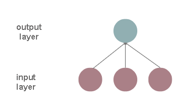
Now let's consider what we actually got from the introduction of neurons and neural networks. Suppose we have three attributes \(x_1, x_2\), and \(x3\). The linear relationship between an attribute and a target variable is mathematically described by the equation \(y = β_0 + β_1x_1 + β_2x_2 + β_3x_3\). If, instead of the parameters β, we write w a instead of β0, write b and move it to the end, we actually get the weight sum \(w_1x_1 + w_2x_2 + w_3x_3 + b\) calculated by one neuron for the signals it receives. This means that if there were no activation function, \(φ\) and neuron would model a linear relationship between attributes (signals) and outputs. This can also be graphically represented by a network consisting of only an input layer with three neurons and an output layer with one neuron, as in the figure below.

If the activation function didn't exist, from a dependency modeling perspective, would adding a new hidden layer make a difference? Let it be a layer of yellow color in the next picture.

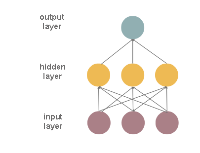
Now each neuron of the hidden layer calculates some linear combination of attributes, and the neuron of the output layer calculates some linear combination of values of the hidden layer. This would mean that our output layer neuron is again calculating some linear combination of attributes, and that we haven't moved much from representing some more complex relationships between attributes and outputs. In addition, we wouldn't move even by adding 100 hidden layers - we'd always be modeling a linear dependence.

 That's why the inclusion of an activation function in the calculations of neurons significantly changes the set of possibilities we have. If we use a nonlinear activation function, we will be able to model some nonlinear relationships between the attribute and the target variable. Thus, the existence of a nonlinear activation function in the hidden layer from the previous example allows the output layer neuron to now compute some nonlinear combination of attributes. In this light, adding new layers makes much more sense. By combining the nonlinearities of multiple layers, we can model complex relationships between attributes and outputs.

 In order to fit all the cubes together, it remains to be discussed what are the nonlinear activation functions that are popular in machine learning. These are the sigmoid function that we got to know in the story of logistic regression, hyperbolic tenges, Rectified Linear Unit (ReLU) and Leaky Rectified Linear Unit (Leaky ReLU). The formulas by which these functions are calculated and their graphs are shown in the figure below. As you can see, these functions are not really linear - their graphics are not real.

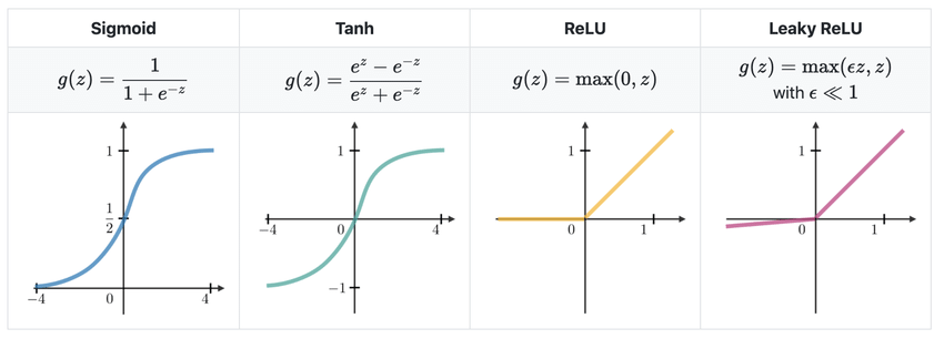
The Most Common Choices of Activation Functions

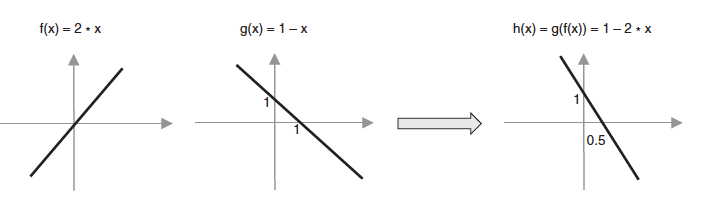
To complete the story of combining different activation functions, let's look at the functions \(f(x)= 2x\) and \(g(x)= 1 − x\). We can see that both functions of a linear function are a variable. By combining them, the composition of the functions, we obtain the function \(g(f(x))= 1 − 2x\), which is also a linear function of a variable. You can see the graphics of all three functions in the image below.

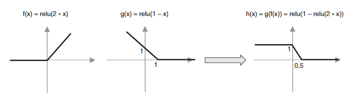
Let us now consider the functions \(f(x)= ReLU(2x)\) and \(g(x)= ReLU(1 − x)\), which differ from the previous functions in that they feature the activation function of a rectified linear unit. Therefore, both functions are nonlinear. By combining them, i.e. By composing them, we get the function \(g(f(x))= ReLU(1 − ReLU(2x))\), which is also nonlinear, and which has a new "form": it allows us to express a slightly different relationship between the input variable and the output.

The choice of the appropriate activation function depends on the nature of the task and some of the properties that the neural network should have during training. How this is done, we will explain in the next lesson.