Completion requirements:
- View
Decision Trees are versatile Machine Learning algorithms that can perform both classification and regression tasks, and even multioutput tasks. They are very powerful algorithms, capable of fitting complex datasets.
A decision tree is a flowchart-like tree structure where an internal node represents a feature(or attribute), the branch represents a decision rule, and each leaf node represents the outcome.
The topmost node in a decision tree is known as the root node. It learns to partition on the basis of the attribute value. It partitions the tree in a recursive manner called recursive partitioning. This flowchart-like structure helps you in decision-making. It's visualization like a flowchart diagram which easily mimics the human level thinking. That is why decision trees are easy to understand and interpret.
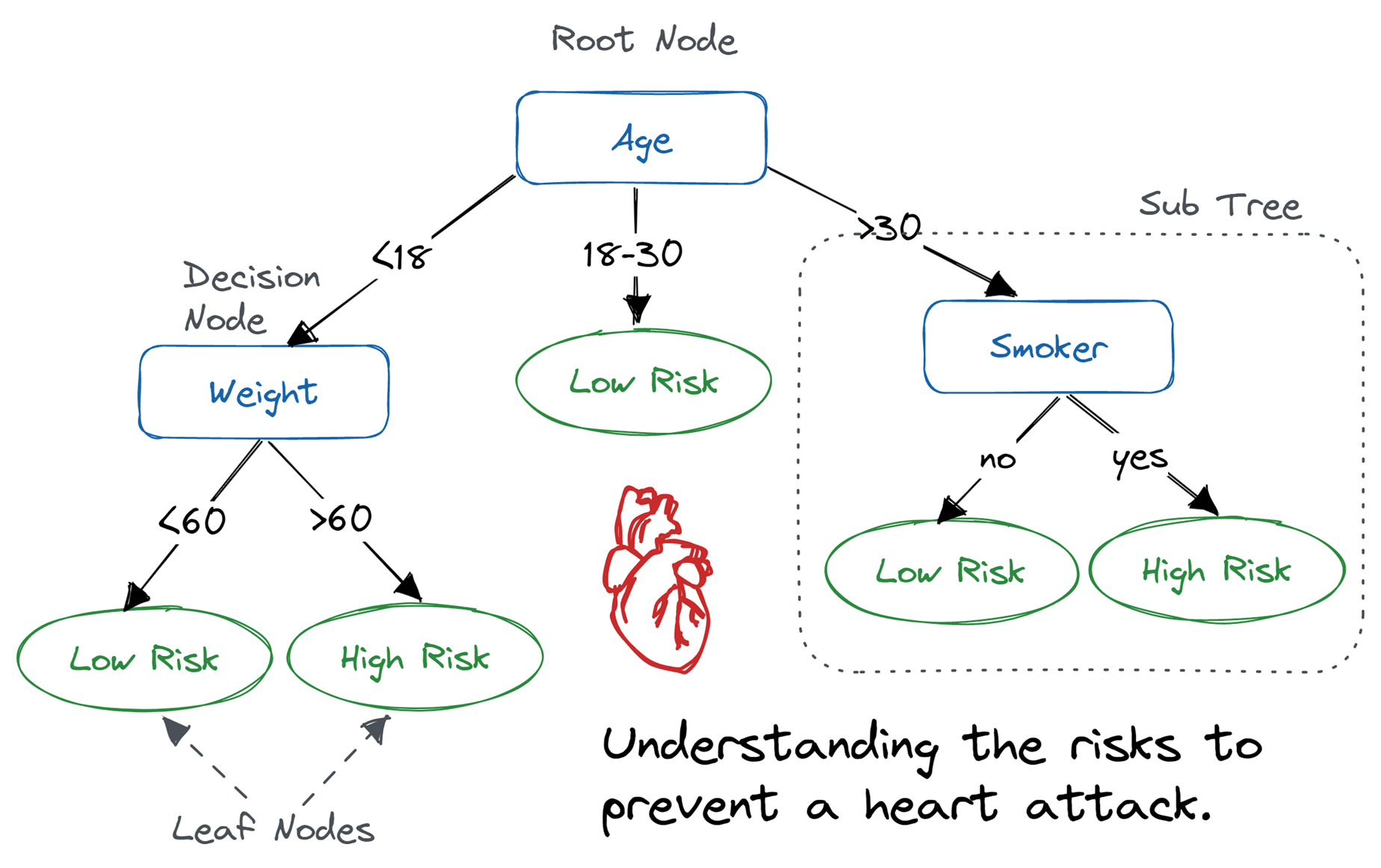
A decision tree is a white box type of ML algorithm. It shares internal decision-making logic, which is not available in the black box type of algorithms such as with a neural network. Its training time is faster compared to the neural network algorithm.
The time complexity of decision trees is a function of the number of records and attributes in the given data. The decision tree is a distribution-free or non-parametric method which does not depend upon probability distribution assumptions. Decision trees can handle high-dimensional data with good accuracy.
How Does the Decision Tree Algorithm Work?
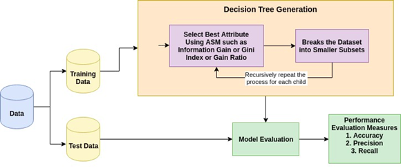
The basic idea behind any decision tree algorithm is as follows:
- Select the best attribute using Attribute Selection Measures (ASM) to split the records.
- Make that attribute a decision node and breaks the dataset into smaller subsets.
- Start tree building by repeating this process recursively for each child until one of the conditions will match:
- All the tuples belong to the same attribute value.
- There are no more remaining attributes.
- There are no more instances.
Attribute Selection Measures
Attribute selection measure is a heuristic for selecting the splitting criterion that partitions data in the best possible manner. It is also known as splitting rules because it helps us to determine breakpoints for tuples on a given node. ASM provides a rank to each feature (or attribute) by explaining the given dataset. The best score attribute will be selected as a splitting attribute . In the case of a continuous-valued attribute, split points for branches also need to define. The most popular selection measures are Information Gain, Gain Ratio, and Gini Index.
Information Gain
Claude Shannon invented the concept of entropy, which measures the impurity of the input set. In physics and mathematics, entropy is referred to as the randomness or the impurity in a system. In information theory, it refers to the impurity in a group of examples. Information gain is the decrease in entropy. Information gain computes the difference between entropy before the split and average entropy after the split of the dataset based on given attribute values. ID3 (Iterative Dichotomiser) decision tree algorithm uses information gain.
Where Pi is the probability that an arbitrary tuple in D belongs to class Ci.
Where:
- Info(D) is the average amount of information needed to identify the class label of a tuple in D.
- |Dj|/|D| acts as the weight of the jth partition.
- InfoA(D) is the expected information required to classify a tuple from D based on the partitioning by A.
The attribute A with the highest information gain, Gain(A), is chosen as the splitting attribute at node N().
Gain Ratio
Information gain is biased for the attribute with many outcomes. It means it prefers the attribute with a large number of distinct values. For instance, consider an attribute with a unique identifier, such as customer_ID, that has zero info(D) because of pure partition. This maximizes the information gain and creates useless partitioning.
C4.5, an improvement of ID3, uses an extension to information gain known as the gain ratio. Gain ratio handles the issue of bias by normalizing the information gain using Split Info. Java implementation of the C4.5 algorithm is known as J48, which is available in WEKA data mining tool.
Where:
- \( \frac{|D_j|}{|D|} \) acts as the weight of the jth partition.
- v is the number of discrete values in attribute A.
The gain ratio can be defined as
The attribute with the highest gain ratio is chosen as the splitting attribute (Source).
Gini index
Another decision tree algorithm CART (Classification and Regression Tree) uses the Gini method to create split points.
Where pi is the probability that a tuple in D belongs to class Ci.
The Gini Index considers a binary split for each attribute. You can compute a weighted sum of the impurity of each partition. If a binary split on attribute A partitions data D into D1 and D2, the Gini index of D is:
In the case of a discrete-valued attribute, the subset that gives the minimum gini index for that chosen is selected as a splitting attribute. In the case of continuous-valued attributes, the strategy is to select each pair of adjacent values as a possible split point, and a point with a smaller gini index is chosen as the splitting point.
The attribute with the minimum Gini index is chosen as the splitting attribute.
Decision Tree Classifier Building in Scikit-learn
Importing Required Libraries
Let's first load the required libraries.
# Load libraries
import pandas as pd
from sklearn.tree import DecisionTreeClassifier # Import Decision Tree Classifier
from sklearn.model_selection import train_test_split # Import train_test_split function
from sklearn import metrics #Import scikit-learn metrics module for accuracy calculation
Loading Data
Let's first load the required Pima Indian Diabetes dataset using pandas' read CSV function. You can download the Kaggle data set to follow along.
col_names = ['pregnant', 'glucose', 'bp', 'skin', 'insulin', 'bmi', 'pedigree', 'age', 'label']
# load dataset
pima = pd.read_csv("diabetes.csv", header=None, names=col_names)
pima.head()
| pregnant | glucose | bp | skin | insulin | bmi | pedigree | age | label | |
|---|---|---|---|---|---|---|---|---|---|
| 0 | 6 | 148 | 72 | 35 | 0 | 33.6 | 0.627 | 50 | 1 |
| 1 | 1 | 85 | 66 | 29 | 0 | 26.6 | 0.351 | 31 | 0 |
| 2 | 8 | 183 | 64 | 0 | 0 | 23.3 | 0.672 | 32 | 1 |
| 3 | 1 | 89 | 66 | 23 | 94 | 28.1 | 0.167 | 21 | 0 |
| 4 | 0 | 137 | 40 | 35 | 168 | 43.1 | 2.288 | 33 | 1 |
Feature Selection
To understand model performance, dividing the dataset into a training set and a test set is a good strategy.
Let's split the dataset by using the function train_test_split(). You need to pass three parameters features; target, and test_set size.
# Split dataset into training set and test set
X_train, X_test, y_train, y_test = train_test_split(X, y, test_size=0.3, random_state=1) # 70% training and 30% test
Building Decision Tree Model
# Create Decision Tree classifer object
clf = DecisionTreeClassifier()

# Train Decision Tree Classifer
clf = clf.fit(X_train,y_train)

#Predict the response for test dataset
y_pred = clf.predict(X_test)
Evaluating the Model
Let's estimate how accurately the classifier or model can predict the type of cultivars.
Accuracy can be computed by comparing actual test set values and predicted values.
# Model Accuracy, how often is the classifier correct?
print("Accuracy:",metrics.accuracy_score(y_test, y_pred))
Accuracy: 0.6753246753246753
We got a classification rate of 67.53%, which is considered as good accuracy. You can improve this accuracy by tuning the parameters in the decision tree algorithm.
Visualizing Decision Trees
You can use Scikit-learn's export_graphviz function for display the tree within a Jupyter notebook. For plotting the tree, you also need to install graphviz and pydotplus.
pip install graphviz
pip install pydotplus
The export_graphviz function converts the decision tree classifier into a dot file, and pydotplus converts this dot file to png or displayable form on Jupyter.
from sklearn.tree import export_graphviz
from sklearn.externals.six import StringIO
from IPython.display import Image
import pydotplus

dot_data = StringIO()
export_graphviz(clf, out_file=dot_data,
                filled=True, rounded=True,
                special_characters=True,feature_names = feature_cols,class_names=['0','1'])
graph = pydotplus.graph_from_dot_data(dot_data.getvalue())
graph.write_png('diabetes.png')
Image(graph.create_png())
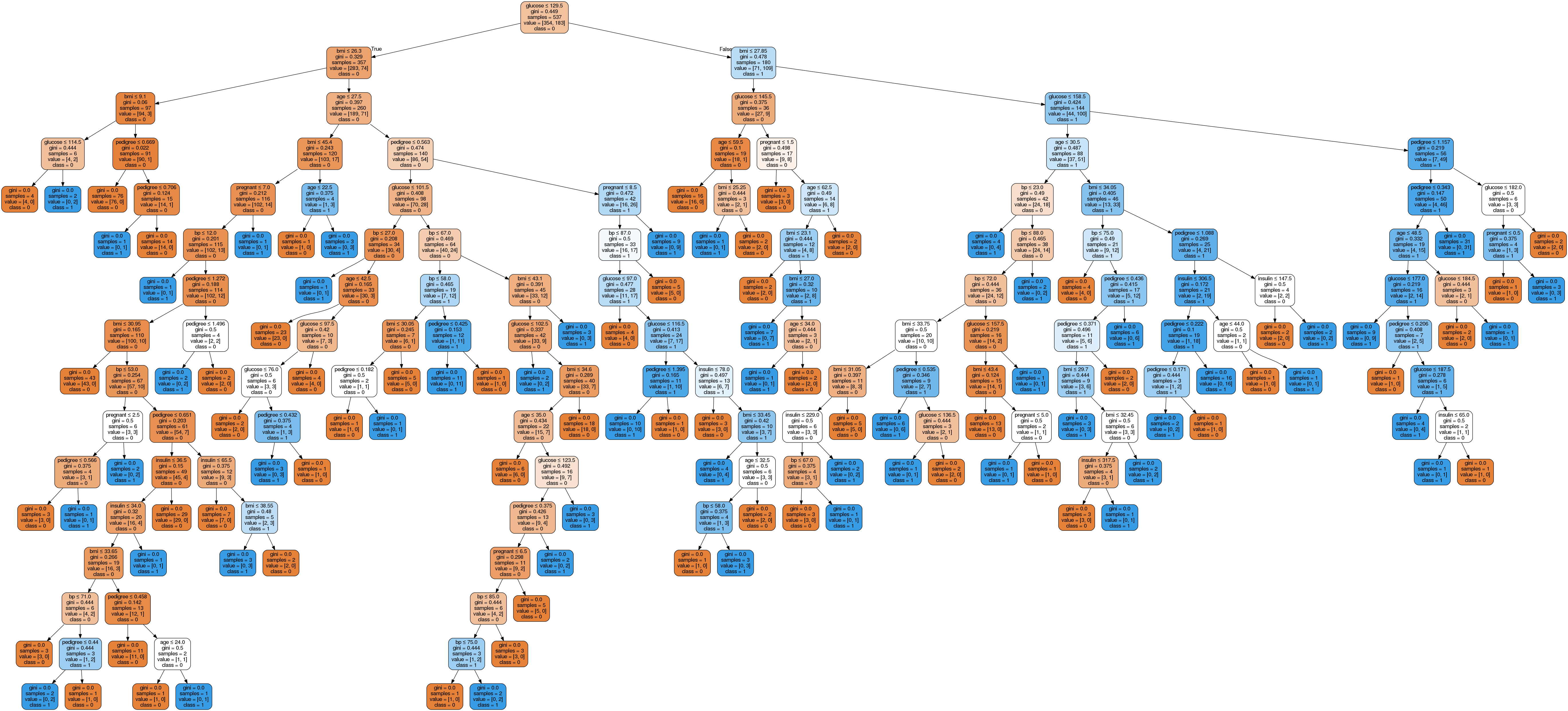
In the decision tree chart, each internal node has a decision rule that splits the data. Gini, referred to as Gini ratio, measures the impurity of the node. You can say a node is pure when all of its records belong to the same class, such nodes known as the leaf node.
Here, the resultant tree is unpruned. This unpruned tree is unexplainable and not easy to understand. In the next section, let's optimize it by pruning.
Optimizing Decision Tree Performance
-
criterion : optional (default=”gini”) or Choose attribute selection measure. This parameter allows us to use the different-different attribute selection measure. Supported criteria are “gini” for the Gini index and “entropy” for the information gain.
-
splitter : string, optional (default=”best”) or Split Strategy. This parameter allows us to choose the split strategy. Supported strategies are “best” to choose the best split and “random” to choose the best random split.
-
max_depth : int or None, optional (default=None) or Maximum Depth of a Tree. The maximum depth of the tree. If None, then nodes are expanded until all the leaves contain less than min_samples_split samples. The higher value of maximum depth causes overfitting, and a lower value causes underfitting (Source).
In Scikit-learn, optimization of decision tree classifier performed by only pre-pruning. Maximum depth of the tree can be used as a control variable for pre-pruning. In the following the example, you can plot a decision tree on the same data with max_depth=3. Other than pre-pruning parameters, You can also try other attribute selection measure such as entropy.
# Create Decision Tree classifer object
clf = DecisionTreeClassifier(criterion="entropy", max_depth=3)

# Train Decision Tree Classifer
clf = clf.fit(X_train,y_train)

#Predict the response for test dataset
y_pred = clf.predict(X_test)

# Model Accuracy, how often is the classifier correct?
print("Accuracy:",metrics.accuracy_score(y_test, y_pred))
Here, we've completed the following steps:
- Imported the required libraries.
- Created a
StringIOobject calleddot_datato hold the text representation of the decision tree. - Exported the decision tree to the
dotformat using theexport_graphvizfunction and write the output to thedot_databuffer. - Created a
pydotplusgraph object from thedotformat representation of the decision tree stored in thedot_databuffer. - Written the generated graph to a PNG file named "diabetes.png".
- Displayed the generated PNG image of the decision tree using the
Imageobject from theIPython.displaymodule.
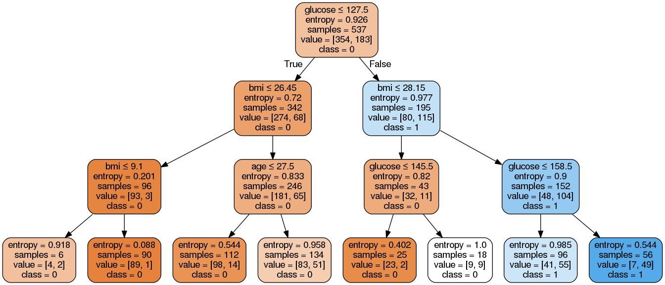
As you can see, this pruned model is less complex, more explainable, and easier to understand than the previous decision tree model plot.
Decision Tree Pros
- Decision trees are easy to interpret and visualize.
- It can easily capture Non-linear patterns.
- It requires fewer data preprocessing from the user, for example, there is no need to normalize columns.
- It can be used for feature engineering such as predicting missing values, suitable for variable selection.
- The decision tree has no assumptions about distribution because of the non-parametric nature of the algorithm. (Source)
Decision Tree Cons
- Sensitive to noisy data. It can overfit noisy data.
- The small variation(or variance) in data can result in the different decision tree. This can be reduced by bagging and boosting algorithms.
- Decision trees are biased with imbalance dataset, so it is recommended that balance out the dataset before creating the decision tree.
Last modified: Sunday, 2 March 2025, 6:42 PM