3.4 Multiple linear regression

In the introductory story about datasets, we saw that a larger number of attributes are used. However, in the story of linear regression, we used only one attribute (the square footage of the property). You're probably wondering what we do when we have multiple attributes and whether we can then apply a linear regression model.

 The linear regression model that is adapted to this scenario is called multiple linear regression and has the form \(y = β_0 + β_1X_1 + β_2X_2 + β_3X_3 +...+ β_nX_n\). Don't be confused by this long expression - now the values \(X_1, X_2, X_3, ..., X_n\) represent the individual attributes and the parameters \(β_0, β_1, β_2, β_3, ..., β_n\) are the parameters of the model. Behind this generalization is again the idea of a linear relationship between the individual attributes and the target variable.

The goal of learning is to determine the values of the parameters \(β_0, β_1, β_2, β_3, ..., β_n\) and thus get an idea of the dependencies. We arrive at them in the same way as with the linear regression that we have come to know (we also say that it is simple): by minimizing the mean square error on the training dataset. The gradient descent technique can be generalized to suit this task setup and can help us find the set of values \(β_0, β_1, β_2, β_3, ..., β_n\) for which the mean square error is the smallest.

In the case of a single-attribute linear regression model, we could also imagine the meaning of the parameters \(β_0\) and \(β_1\): they determined the displacement and slope of the line passing through the data set. Thus, they showed us the strength of the linear dependence between the input and output variables, i.e. how much the value of the output variable y changes when we change the attribute \(x\) by 1. Now that we have more parameters, it is natural to wonder what meaning we can give them. They have the same kind of dependency. If we imagine that only \(β_0\) and \(β_2\): are non-zero parameters, then the relationship between the target variable y and the attribute \(X_2\) is represented by the equation \(y = β_0 + β_2X_2\), i.e. Linear and the same tells us how much the value for the target variable y will change and in which direction when we change the value for \(X_2\) by 1.

 Given that the parameters summarize the knowledge from the data set for us, in the case of multiple linear regression, larger parameter values indicate a greater significance of an attribute on the value of the target variable. In order to be able to track this property, we usually plot the values of the calculated parameters with a column graph. The figure below shows the parameter values of a model that uses a real dataset to predict real estate prices (the popular Boston real estate). Without going into much detail about this set, we can immediately notice that the LSTAT attribute has the most, and negatively, on the value of the target variable, while the RM and RAD attributes have a positive effect, almost equally. Graphics of this type, which can give us some idea of the influence of attributes, are called feature importance graph.

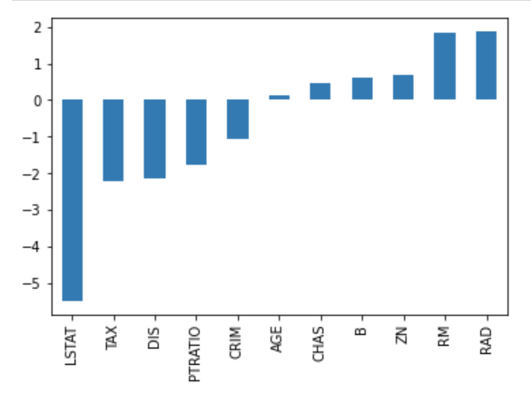
Graph of the importance of multiple regression attributes

Another detail that should be emphasized, so as not to surprise you later, concerns linearity. The linear regression model is linear in terms of parameters . This means that a model whose form \(y = β_0 + β_1X + β_2X^2 + β_3X^3\), in which the degrees of attribute values are figured, would be run as a linear model. It is similar for the model \(y = β_0 + β_1log(X)\), in which the logarithm of the attribute value is figured. You can think of these perhaps unexpected attribute roles as transformations that fix the linear relationship between the attribute and the target variable.