3.2 Gradient Descent

You'll have to imagine something again - this time you're on top of a beautiful mountain. That is not so difficult! The trouble is that now follows the task: to get down to the foot quickly! One way to do this is to first look around and see which direction in your area the mountain is steepest - keep in mind that you need to go down very quickly! Then you can take a careful step in that direction and then stop and look around again. Again, you can see which direction the mountain is the steepest in your area, take a step in that direction and stop. It is clear to you that you can continue to repeat this order of observation, choice of direction and lunge until you reach the foot. There is a refreshment waiting for you for a successfully completed task!

A little physical activity in the middle of a linear regression story doesn't hurt, but you sense that there's something else. The mean square error function depends on the choice of the parameters \(\beta_0\) and \(\beta_0\) - for different combinations of \(\beta_0\) and \(\beta_1\) values, we get different error values. If we plot a graph of this function, for example, along the x-axis we record the values of \(\beta_0\), along the y-axis we record the values of \(\beta_1\), and along the z-axis we record the error values, we get a graph that looks like the one in the figure below. If we mark a random selection of the parameters \(\beta_0\) and \(\beta_1\) with a red dot, in order to get to the point for which the error value is smallest, we really have to go down to the foot of this surface. That is why the "technique" that we developed in the previous example is very relevant. We just need to figure out how to find the steepest directions of descent. Functions will help us with this.

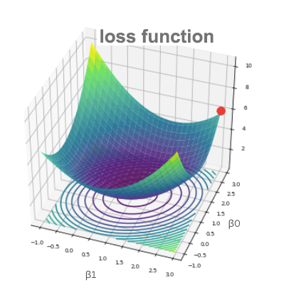
Graph of the Mean Square Error Function

The smallest value of a function is called the minimum.

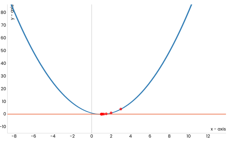
Now let's look at the quadratic function \(f(x)=(x-1)^2\), whose graph is shown in the figure below, and try to reach its minimum with the descent technique - it is at the point \(x=1\) and is 0.

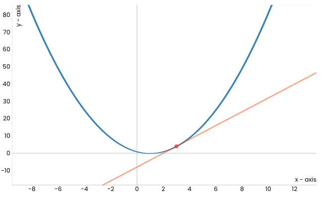
Notice the red dot corresponding to \(x=3\) (randomly chosen) that marks the starting position of the movement towards the minimum of this function. It seems that the orange line marks the steepest direction along which we can start the descent. Interestingly, this line actually represents the tangent of our function at the point \(x=3\). If we take a step along this line, we will find ourselves at a new point. Let's mark its value in red and display it on the graph. It's a little closer to the expected minimum.

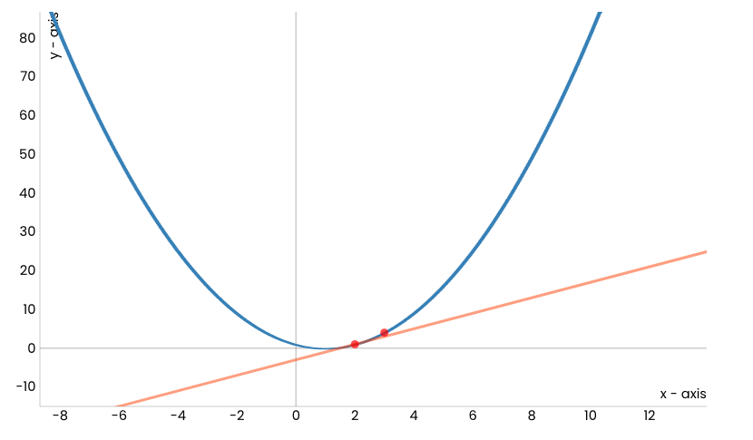
Now we can repeat the process: let's draw a tangent at a new point, and then take a step along that line.

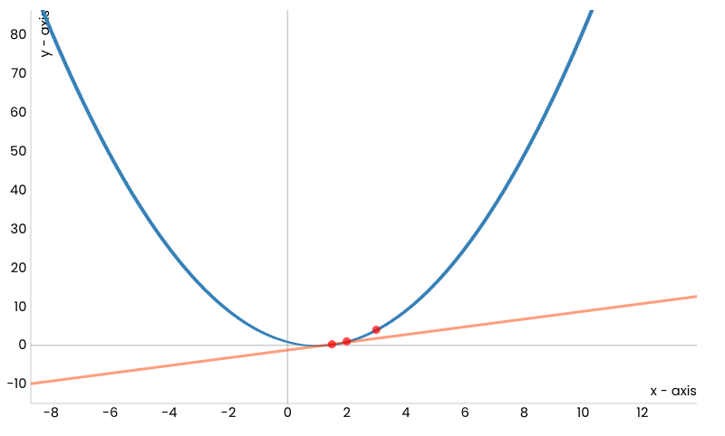
After a certain number of steps, this procedure will bring us to the minimum function, i.e. to the point \(x = 1\).

This section is paired with Jupyter Notebook 05-2-gradient_descent.ipynb . To follow the content further, click on the button   to open the content in Google Colab. If you are viewing the notebooks on your local machine, find the notebook with the same name among the contents and run it. For more detailed instructions, see the Hands-on Zone section and the Jupyter Exercise Notebook lesson.

In the notebook that accompanies this material, you can start the animation yourself and make sure that it is so.

Before we go into more detail about the procedure we have described, let's recall what these real tangents are. For a fixed point \(x\), the coefficient of the direction of the tangent at \(x\) is equal to the value of the first derivative of the function at \(x\). The first derivative of our function is the function \(f′(x)= 2x − 2\) and at the initial point \(x = 3\) the value of the derivative is \(f′(x)= 4\). This means that the tangent has the equation \(y = 4x − 8\) (the number -8 is obtained from the condition that this line must contain a point (3, 4 )). That is why we can also say that the tangent has a direction corresponding to the derivative of a function at a certain point, and for the movement itself in that direction that the movement along the direction of the derivative is at that point. Now the dilemma is whether we move along or down, i.e. Are we going in the opposite direction, or are we going in the opposite direction? Well, since we want to go down to the minimum, we need to follow the direction opposite to the direction of the derivative of the function.

 If we now denote the starting point with \(x_0\), we get a new point \(x_1\) by taking a step along the direction of the derivative of the function at the point \(x_0\). If we denote the length of the step with \(α\), we calculate the value of the new point \(x_1\) as \(x_1 = x_0 − αf′(x_0)\). Since we repeat the procedure, we calculate the value of the point \(x_2\) as \(x_2 = x_1 − αf′(x_1)\) and continue with the calculations \(x_3 = x_2 − αf′(x_2)\), \(x4 = x_3 − αf′(x_3)\), ... Repeat the procedure until for two consecutive values, say \(x_{34}\) and \(x_{35}\), the values of the function are close enough, i.e. while the absolute value of the difference \(f(x_{35})− f(x_{34})\) is not less than some predetermined precision, say 0.001. Thus, computationally, we can approach the concept of convergence in mathematics.

The value α we introduced is called the learning rate and represents a very important parameter of the algorithm that we have described. If the values for α are very small, it will take us a long time to reach the minimum. On the other hand, if the values for α are very high, it can happen that we skip the minimum or fall into a zigzag trap by constantly jumping around it! Look at the image below!

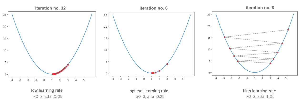
The Impact of Learning Step Choices

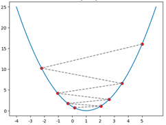
Zigzag lock

Be sure to check both of these behaviors yourself in the companion notebook using the different settings for the learning step in the animation.

The algorithm we have described is called Gradient Descent and despite its simplicity, it is one of the most important algorithms in machine learning because it makes it possible to find the smallest value of an error function. There are many details about this algorithm that we won't go into about the properties of the functions to which this algorithm can be successfully applied, the numerical calculation of the derivative, and the selection of learning steps. All of them must be considered during the practical application of the algorithm.

The algorithm itself is not unpleasant to program, so we will embark on an adventure. We need a function f, which will calculate the value of a given function, and a function f_izvod, which will calculate the value of the derivative of a given function. We need to define both the alpha learning step and the stop criteria: we will suspend the procedure when the values of the function in two successive iterations are close enough (the difference between their values is less than some predetermined epsilon accuracy) or when we reach a finite number of iterations max_broj_iteracija (we also need to make sure in cases of inappropriate learning step choices).

Follow the code block. The algorithm started by setting a starting point. Since the point at which we move by the gradient descent algorithm is the starting point of the next step, we use the x_staro and x_novo markers to mark them in successive steps. The report that we create at the end of the function contains information about whether the algorithm has stopped, how many steps it takes, i.e. iteration needed and what value it found.

def gradient_descent(f, f_derivative, x, alpha, epsilon, max_iterations):

    # set the initial value for x
    x_old = x

    # in each iteration ...
    for i in range(0, max_iterations):

        # calculate the current value for x
        x_new = x_old - alpha * f_derivative(x_old)

        # and then check if the stopping criterion is met
        if np.abs(f(x_new) - f(x_old)) < epsilon:
            break

        # if the criterion is not met, prepare x for the next iteration
        x_old = x_new

    # at the end of the whole process, prepare a report with information:
    # whether the algorithm stops,
    # how many iterations it lasted,
    # and what value of x was found
    report = {}
    report['stops'] = i != max_iterations
    report['number_of_iterations'] = i
    report['x_min'] = x_old

    return report

 The function and its derivation can be defined by the following Python blocks:

def f(x):
   return (x-1)**2

def f_izvod(x):
   return 2*x-2

After running the gradient_descent function for the values of the arguments x0 = 3, alpha = 0.1, epsilon = 0.001, and max_broj_iteracija = 100, we get that the minimum of the function is 1.0048, which we can confirm. You can also run the code yourself and make sure that you get the result. Don't forget to examine how the results change if other argument values are selected.

Now we can return to the problem of finding the parameters \(\beta_0\) and \(\beta_1\) of linear regression for which the value of the mean square error should have the smallest value. The mean square error function is a function of two variables - it depends on both the value of the parameter \(\beta_0\) and the value of the parameter \(\beta_1\). When working with functions of multiple variables, in general with n variables \(x_1,  x_2, x_3, ..., x_n\), the derivative that we used in the gradient descent algorithm is generalized by a vector of partial derivatives - for each of the variables we calculate the derivatives individually. For example, for a function \(\frac{1}{2} (x_1^2 + 10x_2^2)\), the derivative of the variable \(x_1\) is obtained by declaring the variable \(x_2\) as a constant and then applying the standard rules for calculating the derivative that bring us to \(\frac{1}{2} ⋅ 2 ⋅ x_1 = x_1\). On the other hand, the derivative of the variable \(x_2\) is calculated by declaring the variable \(x_1\) as a constant and applying the standard rules for calculating the derivative. Now we get \(\frac{1}{2} ⋅ 10 ⋅ 2 ⋅ x_2 = 10 ⋅ x_2\). Now we get that the vector of the derivative by individual variables (such derivatives are called partial) is the vector \([x_1,10 ⋅ x_2]\). In mathematics, and even in machine learning, these vectors are called gradients, hence the name of the algorithm itself. To denote gradients, we use the symbol triangle down, \(∇\) called nabla. Thus, the precise notation of the gradient of the starting function f′ would be \(∇ f(x_1, x_2 )= [x_1 ,10 ⋅ x_2 ]\) and would allow us to keep track of which directions of the lead we should move individually during the descent.

The other steps of the gradient descent algorithm do not differ much in the case of multivariate functions: we expect the algorithm to stop after the desired accuracy has been achieved, or after a certain number of iterations have been performed.

Now that we understand how gradient descent works for functions of multiple variables, let's go back to calculating the parameters \(\beta_0\) and \(\beta_1\). We said that the equation of the mean square error is \(\frac{1}{N} \sum\limits_{i = 1}^{N}(yi −(\beta_0 + \beta1xi))^2\). Since this is a function for which we need to find the minimum, if we roll up our sleeves and check, we get that the derivative of the mean square function by \(\beta_0\) is exactly \(\frac{2}{N} \sum\limits_{i = 1}^{N}(\beta_0 + \beta_1x_i − y_i)\) and the derivative by \(\beta_1\) is exactly \(\frac{1}{N} \sum\limits_{i = 1}^{N}(\beta_0 + \beta_1x_i − y_i) ⋅ x_i\) . These derivatives indicate which directions we should move along and how much we should correct the values for \(\beta_0\) and \(\beta_1\) in each step of the gradient descent iteration.

In the notebook, you can also see how these values are calculated through code, and then go through the entire process of custom gradient descent. For the real estate set we have introduced, we will arrive at the values of \(\beta_0 = 2.056\) and \(\beta_0 = 1.198\).

We have said that there are certain prerequisites that a function needs to satisfy in order for its minimum to be found by the gradient descent technique (it is necessary for the function to be differentiable). It is also important to know that in general a local minimum is reached in this way. For example, the function in the figure below has several local minimums and only one global minimum . In some cases, for example, when a function is convex, the local and global minimums coincide, so we always arrive at the desired solution, the global minimum. The squared error function is convex by the parameters \(\beta_0\) and \(\beta_1\).

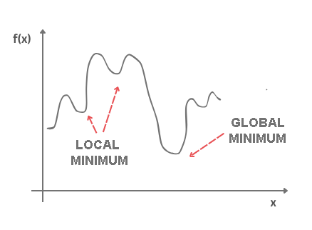
Local and global minimums.

The field of mathematics that deals with finding the maximum and minimum values of functions (we call them optimums by one name) is called mathematical optimization . Gradient descent is only one algorithm from the palette of this field.