Completion requirements:
- View
Let's go back to the example we used to introduce the data-driven programming paradigm. In the dataset, we had information about the square footage of the properties and their prices, and our task was to learn the connection between these values so that we could estimate prices for new properties.
For the sake of simplicity, let's have a training set that contains 10 instances, which are listed in the table below:
| Square Footage (m2) | Real estate Prices (1000€) |
| 43 | 60 |
| 25 | 32.1 |
| 66 | 88.4 |
| 80 | 111.4 |
| 105 | 120.32 |
| 70 | 72.1 |
| 40 | 46.3 |
| 85 | 90.1 |
| 84 | 99.6 |
| 102 | 139.2 |
We can also display these images graphically. Along the x-axis, we will set the values of square footage, along the y-axis the values of real estate prices and mark the pairs of values with blue circles.
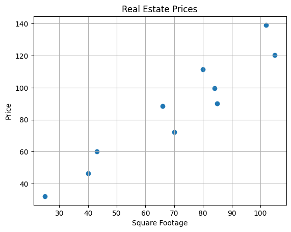
Let us choose for the model a function that relates the real estate square footage x and the real estate prices y with the equation \(y = \beta_0 + \beta_1x\), where \(\beta_0\) and \(\beta_1\) represent unknown parameters. This is the so-called linear model , and since we use it to solve the regression problem, we also call it a linear regression model . Note that this is actually a line equation \(y = kx + n\), where the coefficient of the line line is denoted by \(\beta_1\) and the free term is denoted by \(\beta_0\). The motivation for introducing this model lies in the fact that The dots follow the imaginary diagonal of the quadrant, perhaps slightly lowered.
This section is paired with Jupyter Volume 05-1-linear_regression.ipynb . To follow the content further, click on the link and then on the button  to open the content in Google Colab . If you are viewing the notebooks on your local machine, find the notebook with the same name among the contents and run it. For more detailed instructions, see the Hands-on Zone section and the Jupyter Exercise Notebook lesson.
Your task is to load the real estate data set in the companion notebook and select the values of the parameters \(\beta_0\) and \(\beta_1\) that you think best match this data. You can adjust them by moving the sliders left and right. Remember the values you have chosen and what ideas guided you when determining the parameters.
You've probably tried to get the right one that comes as close as possible to the given points and makes as few deviations as possible. You were equally satisfied with some parameter choices, while some were really bad. And from the point of view of machine learning, we try to find the values of the parameters \(\beta_0\) and \(\beta_1\) for which we make the smallest error, but we have to define exactly what the error actually is. Here's how we're going to do it.
Suppose the selected values are \(\beta_0= 6.3\) and \(\beta_1= 1.02\). Now let's expand the data table with a column with the values calculated by this linear regression model for the quadrature values we have. From the angle of the model, we represent them with the size x.
|
Square Footage |
Real estate Prices (1000€) |
Model price \(y = 6.3 + 1.02x\) (1000€) |
| 43 | 60 | 50.16 |
| 25 | 32.1 | 31.8 |
| 66 | 88.4 | 73.62 |
| 80 | 111.4 | 87.9 |
| 105 | 120.32 | 113.4 |
| 70 | 72.1 | 77.7 |
| 40 | 46.3 | 47.1 |
| 85 | 90.1 | 93 |
| 84 | 99.6 | 91.98 |
| 102 | 139.2 | 110.34 |
The difference between the values that are expected (known in the data set) and the values that we have calculated (remember to call them predictions) is an error. Now let's calculate all the errors and record them in the table.
|
Square Footage |
Real estate Prices (1000€) |
Model price \(y = 6.3 + 1.02x\) (1000€) |
Model error |
| 43 | 60 | 50.16 | 9.84 |
| 25 | 32.1 | 31.8 | 0.3 |
| 66 | 88.4 | 73.62 | 14.78 |
| 80 | 111.4 | 87.9 | 2.53 |
| 105 | 120.32 | 113.4 | 6.92 |
| 70 | 72.1 | 77.7 | -5.6 |
| 40 | 46.3 | 47.1 | -0.8 |
| 85 | 90.1 | 93 | -2.9 |
| 84 | 99.6 | 91.98 | 7.62 |
| 102 | 139.2 | 110.34 | 28.86 |
To make it easier to track the behavior of the errors, in the image below, their values are shown by blue dotted lines.
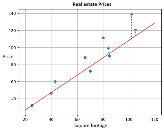
In order to get an idea of the total error of the model, it is unwise to add the individual errors, since some error values are positive and some values are negative. Therefore, we can square them and add them together - this will give us stronger information about the size of the error, regardless of whether it is positive or negative. If we divide the resulting sum by the number of instances in the set, Let's get an idea of the average error of the model. In our case, it is: \((9.84^2+0.32^2+14.782^2+23.52^2+6.92^2+(-5.6)^2+(-0.8)^2+(-2.9)^2+7.62^2+28.86^2)/10=184.687\)
The error of the linear regression model calculated in this way is called the mean square error (MSE). For fixed values of the parameters \(\beta_0\) and \(\beta_1\), the calculation procedure we have described can be abbreviated by the formula \(\frac{1}{N}\sum\limits_{i = 1}^{N}(y_i-(\beta_0+\beta_1x_i))^2\). In it, the pairs \(x_i,y_i\) correspond to the individual instances, the square footage of the properties xi and their prices yi, and the number n indicates the total number of instances. That's 10 in our case. The expression figured in the sum represents the difference between the expected yi and the calculated \(\beta_0+ \beta_1x_i\) values.
The squared error is the error that we always pair with the linear regression model, and that we want to minimize as much as possible by choosing the rulex parameters \(\beta_0\) and \(\beta_1\). From the experience of setting the parameters, you have seen that this is not a very easy task. Fortunately, there are mathematical techniques that can help us with this. To figure out how to do this, let's move on to the next lesson on gradient descent.
Last modified: Thursday, 26 June 2025, 10:39 PM