2.8 Creating a Representation of a Dataset

Preparation of numerical attributes

When working with numerical attributes, we encounter quantities that are expressed on different scales of values. For example, in a single set of medical data, there may be laboratory analyses with values ranging from 0 to 1 and information about the patient's height expressed in centimeters, from 100 to 250, which is significantly higher. Many machine learning models are sensitive to the presence of these attributes and therefore take longer to find a solution. It's not easy to understand the results that come with this kind of work. That's why when working with numeric data, we use normalization techniques that help us bring a set of attribute values to the same ranges of values.

One such normalization is min-max normalization. To clarify how it is performed, suppose that we need to normalize the value of the attribute X to express the height of the patients. Let Xmax = 180 represent the maximum height of the patients and Xmin = 110 the smallest. The normalization of min-max  is carried out by applying the formula (x − Xmin)/(Xmax − Xmin) to each value of the attribute x. If x = 165, the new normalized value will be x′= (165 − 110)/(180 − 110) = 0.786. In this way, The value of the attribute is reduced to a range from 0 to 1.

One of the most important aspects of normalization is standardization. It involves centering the attribute value around zero and scaling to unit variance. To clarify how it is carried out, we can again assume that we need to normalize the value of the X attribute, which expresses the height of patients. Let now Xmean = 153.2 the mean height in the data set and σ = 40.23 the standard deviation. Standardization is accomplished by applying the formula (x − Xmean)/σ to each value of the attribute x. The new standardized value for a patient whose height is x = 165 is now x′= (165 − 153,2)/40.23 = 0.293.

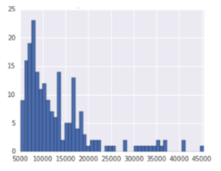
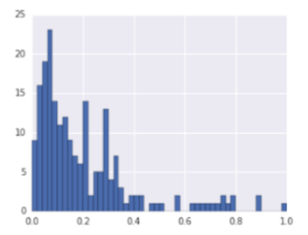
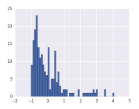
The Effect of Normalization and Standardization on a Data Set

Preparation of categorical attributes

Since machine learning algorithms can only be applied to numbers, categorical attributes require special preparation. We have said that they represent quantities that have a finite number of values and that they often appear in the form of string. Some of the examples we have mentioned are the name of the color, the sex of the patient, and the month of the year.

If an attribute has only two values, for example, representing the sex of a patient, its values are usually mapped to the numbers 0 or 1. For example, the value "female" can be mapped to the number 1, and the value "male" to the number 0. These attributes are otherwise called binary attributes.

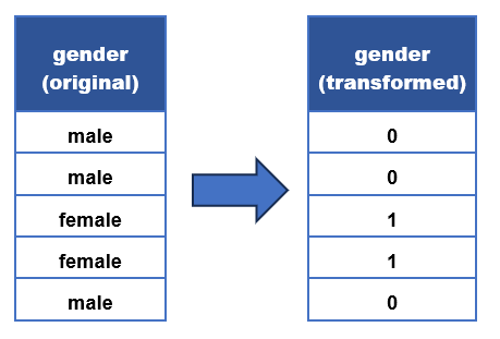
Example of value mapping

For attributes that can have multiple values, we use one-hot coding. To clarify its meaning, we can look at an attribute that represents a color, which can have three values: red, yellow, and green. The idea is to represent the default color attribute using three new attributes, each of which will correspond to one of the values that the color can take: red, yellow and green (look at the picture, this was a complicated sentence). This further means that we will transform each of the values of the initial attribute into a triplet of values, namely the value of red into a triplet of 1 , 0, 0, the value of yellow into a triplet of 0 , 1 , 0, and the value of green into a triplet of 0 , 0 , 1 . The triplets, as we can see, consist of zeros and exactly one unit in the column that corresponds to the value of the attribute.

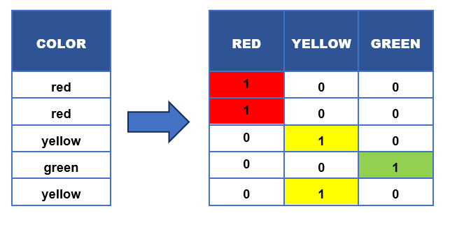
Example of one-hot coding

Representation of the dataset

After the step of transforming attributes, we arrive at the final form of data that we can use to run learning algorithms. This final form is called the representation of the data set . In the story so far, we have covered, first of all, how to arrive at the representation of tabular data. And for all other types of data such as images, audios, text, video-content, but also complex structures such as graphs, We need to create appropriate representations. In the section on neural networks, we will learn about some other ways of creating representations.