15. Exploring Artificial Intelligence

15.  Exploring Artificial Intelligence

15.1  Hardware and Software Support for AI

Recent models of the Raspberry Pi processor include multiple ARM cores. Despite its respectable hardware capabilities, the Raspberry Pi may struggle with the computational demands of more demanding artificial intelligence (AI) applications. For more demanding applications, there is a Raspberry Pi add‑on board — referred to as a HAT (Hardware Attached on Top) that provides an NPU (Neural Processing Unit) to accelerate machine learning computations. The Raspberry Pi AI HAT+ provides a high‑performance, power‑efficient AI processor for the Raspberry Pi 5. Besides hardware support, there are a wide variety of powerful machine learning libraries which can be used with the Raspberry Pi, including scikit‑learn and LiteRT. Python includes a number of powerful supporting libraries, such as Matplotlib and plotly for plotting,NumPy for providing fast operations on arrays, and Pandas for data analysis and manipulation. The following sections provide examples of some of these libraries in action.

 

15.2  SciKit Learn

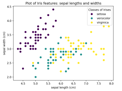
SciKit Learn is an open source machine learning library that works with Python. SciKit Learn provides many different features, including regression and clustering algorithms, Principal Component Analysis (PCA), Linear Discriminant Analysis (LDA), and Support Vector Machines (SVMs). All forms of machine learning require a dataset which is used for training. SciKit includes a selection of toy datasets that can be used to experiment with the machine learning libraries. The following sections demonstrate PCA and SVMs using the classic iris flower dataset which is part of the collection of toy datasets. This iris dataset was originally compiled by biologist Ronald Fisher in a wellknown 1936 paper. This dataset comprises samples of three species of the Iris flower (Iris setosa, Iris virginica, and Iris versicolor) and measurements of the length and the width of both the sepals1 and the petals. The SciKit Learn library includes this iris dataset for testing and demonstration purposes. The followig Python code uses Matplotlib to plot the sepal width versus the sepal length for each of the three iris classes in the dataset.

from sklearn import datasets

import matplotlib.pyplot as plt

# Load the classic iris dataset

iris = datasets.load_iris()

# Plot sepal lengths vs. widths for irises in dataset

fig, ax = plt.subplots()

scatter = ax.scatter(iris.data[:, 0], iris.data[:, 1], c=iris.target)

ax.set_title("Plot of Iris features: sepal lengths and widths")

ax.set(xlabel=iris.feature_names[0], ylabel=iris.feature_names[1])

fig = ax.legend(scatter.legend_elements()[0], iris.target_names, loc="best

", title="Classes of Irises")

plt.show()

Running this code results in the following plot of the iris dataset:

 

 

 

 

15.3    SVM Image Classification

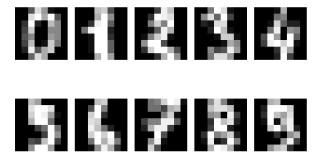
The following example is inspired by the SciKit example on recognizing hand‑written digits and uses the hand‑written digits dataset from the UC Irvine machine learning repository. This dataset has 1797 image samples comprised of an 8𝑥8 array of pixels with 10 classes where each class refers to one digit (0‑9). A short Python program to load the hand‑written digits dataset and display them is shown below:

import matplotlib.pyplot as plt

from sklearn import datasets, metrics, svm

from sklearn.model_selection import train_test_split

 

# load hand-written digits dataset

digits = datasets.load_digits()

 

# display a sample of ten hand-written digits in the dataset

fig, axes = plt.subplots(nrows=2, ncols=5)

for ax, digit in zip(axes.flatten(), digits.images):

    ax.set_axis_off()

    ax.imshow(digit,cmap='gray')

fig.tight_layout()

plt.show()

The plot showing ten hand‑written digits in the dataset is shown below.

We can split the hand‑written digits dataset into two sets: a training set and a set for testing. SciKit has a function for taking the larger digits dataset and splitting it in half into training and test sets as follows:

X_train, X_test, y_train, y_test = train_test_split(X, y, test_size=0.5)

 

where X is an array of of the features and y is a vector of labels that classify the data. Hence we can proceed to train an SVM using half the dataset for training and then use the remaining half of the dataset for testing. The accuracy of the SVM can be determined by comparing the digits predicted by the SVM with the actual labels for the hand‑written digits and the recognition rate can be reported. The recognition rate is the total number of correctly identified digit images divided by the total number of test images. The following code defines an SVM classifier based on half of the dataset and then determines the recognition rate using the other half of the dataset as test images.

import matplotlib.pyplot as plt

from sklearn import datasets, metrics, svm

from sklearn.model_selection import train_test_split

 

# Read digits and reshape digits as a vector of images

digits = datasets.load_digits()

n_samples = len(digits.images)

data = digits.images.reshape((n_samples, -1))

 

# Create a support vector machine classifier

svm = svm.SVC()

# Split the dataset: half for training and half for testing

X_train, X_test, y_train, y_test = train_test_split(

data, digits.target, test_size=0.5, shuffle=False)

 

# Train on hand-written digits in the training set

svm.fit(X_train, y_train)

# Predict the value of the digit using the testing set

predicted = svm.predict(X_test)

 

# compute the recognition rate

matches = 0

for x in range(len(y_test)):

if y_test[x] == predicted[x]:

matches += 1

recognition_rate = (matches/len(y_test)) * 100;

print(f'Recognition rate: {recognition_rate:.2f}%')

 

The output of this code shows the following:

Recognition rate: 96.11%

This indicates a respectable recognition rate using an SVM for handwritten digit classification. For more details, we can plot a confusion matrix to visualize the accuracy of a machine learning algorithm. The confusion matrix is organized into rows and columns: each row represents each of the classes in a dataset and each column represents the predictions that were made. Ideally, the actual classes and the predictions will perfectly align such that the diagonal of the confusion matrix is populated with 100’s and with 0’s everywhere else. The diagonal martix corresponds to true recognition rates whereas all other cells represent the occurrences of false classifications.