Exercise 10: Training neural networks

TensorFlow Playground

Now that you know what neural networks are and how they are trained, you can also try to build and train your own network!

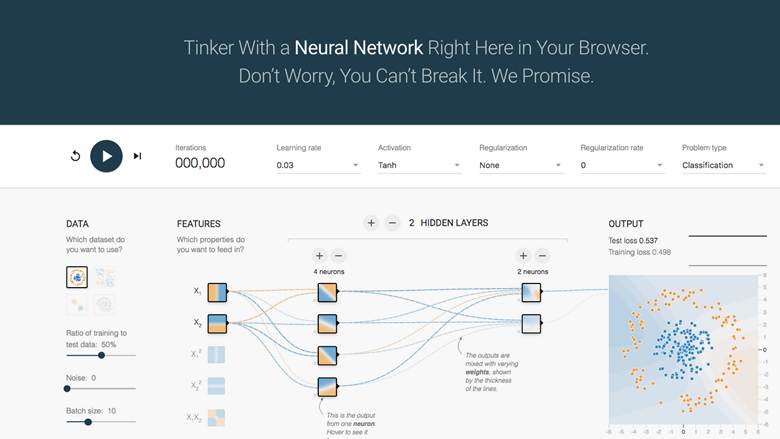
TensorFlow Playground is a graphical environment that will bring you closer to what it actually looks like to train a neural network. You can access it at https://playground.tensorflow.org/ and then continue reading and following along. You don't need a special account or additional software, everything will be executed in your browser. In the window that will be waiting for you, you will immediately see many squares representing neurons and lines representing the connections between them!

The world's most promised land, the 2000s, is the 1000-day day of the 2016 World's Day.

At the top of the   TensorFlow Playground  page, there is a bar that allows you to select the type of task, and then, once you have created a network that solves the problem, you can start training it. You can select the task type, which can be classifying or regression, in  the  Problem type  field  on the far right. Through  the  Learning rate  field,  you can influence the size of the learning step used to determine the best parameter values. In the   Activation   you can choose one of the offered activation functions. The   Regularization   and   Regularization rate  fields  affect the regularization of individual layers of the neural network, similar to the lesson on regularization and the example of linear regression. The training of the network itself is started by clicking on the arrow on the left. The number of training epochs will be printed in the   Iterations  field.

Home bar with options for setting up training

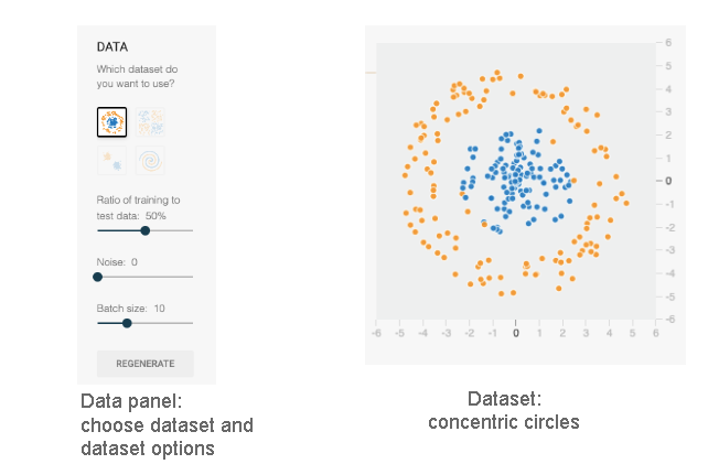
For starters, you can try one of the offered classification tasks. All classification tasks are binary classification tasks, there are four of them in total and they are represented by icons that describe the data sets used in them. Instances that belong to a positive class are colored blue while instances that belong to a negative class are colored orange. You can select sets in the Data sectionOn the left side of the screen. For the exercise, we will initially choose a set represented by concentric circles - the remaining sets are a spiral, four quadrants corresponding to the task of learning exclusive disjunction, and two clusters of data. With the settings in this section, you can also influence the scale of the training set and the test set (by default, these two sets are equal in size) and the level of class overlap (the Noise  parameter). The size of the training packet is set to 10 by default (Batch size  parameter).

The Features section     refers to the input layer and the attributes of the mesh. Since the sets with which the sets of points are in the plane, the \(x_1\) attribute represents the value  of  \(x\)  coordinates and the \(x_2\) attribute  represents  the value of \(y\)  coordinates. It is also possible to select the \(x_1^2, x_2^2, x_1x_2\), as well as \(sin(x_1)\) and \(sin(x_2)\) attributes.

You  can control the number of layers of the neural network with the option   Hidden layers. Clicking on the + button adds a new hidden layer, while clicking on the - button deletes the hidden layer. The number of neurons in individual layers is also controlled by clicking on the + and - buttons. The network that is created in this way is a fully connected neural network. The connections between neurons are shown by dotted lines and their color and thickness are aligned with the values of the parameters that accompany them. By clicking on each of the The value of the parameter can be set individually.

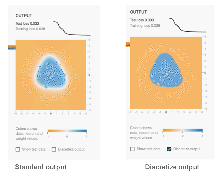
Once you've created the grid, you'll need to click on the arrow to start training. In the panel on the right called   Output,  you'll be able to track the success of your training session visually or by plotting the error curves and displaying their values.

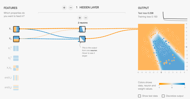
The problem with the concentric data circles that we have chosen for the exercise is not linear - we cannot draw the lines that separate the set of blue and the set of orange instances. Therefore, we need to learn a more complex nonlinear model. We can first try a network that has inputs \(x1\) and \(x2\) and one hidden layer with two neurons that use the ReLU activation function. We will notice that after an epoch the network stagnates with learning, so if we stop it after 500 epochs,  We get an image like in the picture below. The problem itself is not ideally solved because there are no clear boundaries between classes. We can see that the first neuron of the hidden layer has learned to classify instances into left and right (square  ), and the second neuron into those below and above the main diagonal (square  ), so that by combining this knowledge we get a boundary as in the figure. By staying on two neurons and trying out other activation functions, the results will not be satisfactory (be sure to check that!).

 If we now create a network that has inputs \(x_1\) and \(x_2\) and one hidden layer with three neurons using the ReLU activation function, we get a representation like the image below. Now we are able to separate the instances more finely - the first neuron has learned to perceive those in the lower right corner, the second to separate them horizontally (slightly obliquely), and the third vertically (slightly obliquely). All this knowledge is also conditioned by the nature of the activation function that we used. By combining them, we can certainly reach a better boundary between classes.

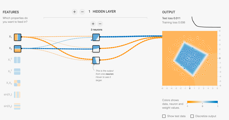
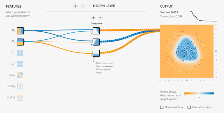
Let's try the same combination, but using sigmoid activation. In a similar number of epochs, we have reached a more oval border. We can also see that now neurons have learned to distinguish instances according to some slightly different criteria, and just as successfully.

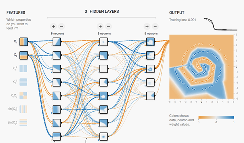
There are many more networks that can solve this task keep experimenting and discover your network. At the end of the exercise, you can leave the spiral task because it is the most challenging. Here's what a network that follows him might look like!

In practice, libraries such as TensorFlow,Hard,PyTorch,JAX and others. Through their API, they offer functionalities that describe the layers of the network, adjust optimization algorithms and monitor the entire training process. In addition to these core functionalities, libraries also define techniques for monitoring readaptation, measures for evaluating models, as well as mechanisms for controlling and allocating hardware resources. These libraries are usually paired with libraries that show the entire training process more finely graphically. Libraries are, for example TensorBoard and Weights & Biasis. There are also many tools tailored to specific tasks.