Exercise 6: Logistic Regression

Logistic Regression

Here's a simple Jupyter Notebook exercise for students to learn about classification using logistic regression. This exercise will guide them through loading a dataset, training a logistic regression model, and evaluating its performance.

Exercise: Classification Using Logistic Regression

Objective:
Load a dataset. Train a logistic regression model. Evaluate the model's performance.
Prerequisites:
Install the scikit-learn library. Use a simple dataset like the Iris dataset.

Step 1: Install Required Libraries:

%pip install scikit-learn

Step 2: Import Libraries:

import numpy as np
import matplotlib.pyplot as plt
from sklearn import datasets
from sklearn.model_selection import train_test_split
from sklearn.linear_model import LogisticRegression
from sklearn.metrics import accuracy_score, confusion_matrix, classification_report

Step 3: Load the Dataset:

# Load the Iris dataset
iris = datasets.load_iris()
X = iris.data
y = iris.target

# Use only two classes for binary classification
X = X[y != 2]
y = y[y != 2]

Step 4: Split the Dataset:

# Split the dataset into training and testing sets
X_train, X_test, y_train, y_test = train_test_split(X, y, test_size=0.3, random_state=42)

Step 5: Train the Logistic Regression Model:

# Initialize and train the logistic regression model
model = LogisticRegression()
model.fit(X_train, y_train)

Step 6: Make Predictions:

# Make predictions on the test set
y_pred = model.predict(X_test)

Step 7: Make Predictions:

# Evaluate the model's performance
accuracy = accuracy_score(y_test, y_pred)
cm = confusion_matrix(y_test, y_pred)
cr = classification_report(y_test, y_pred)
print(f'Accuracy: {accuracy}')
print('Confusion Matrix:')
print(cm)
print('Classification Report:')
print(cr)

Step 8: Visualize the Results:

# Visualize the confusion matrix
plt.figure(figsize=(8, 6))
plt.imshow(cm, interpolation='nearest', cmap=plt.cm.Blues)
plt.title('Confusion Matrix')
plt.colorbar()
tick_marks = np.arange(len(iris.target_names[:2]))
plt.xticks(tick_marks, iris.target_names[:2], rotation=45)
plt.yticks(tick_marks, iris.target_names[:2])

fmt = 'd'
thresh = cm.max() / 2.
for i, j in np.ndindex(cm.shape):
    plt.text(j, i, format(cm[i, j], fmt),
             ha="center", va="center",
             color="white" if cm[i, j] > thresh else "black")

plt.ylabel('True label')
plt.xlabel('Predicted label')
plt.tight_layout()
plt.show()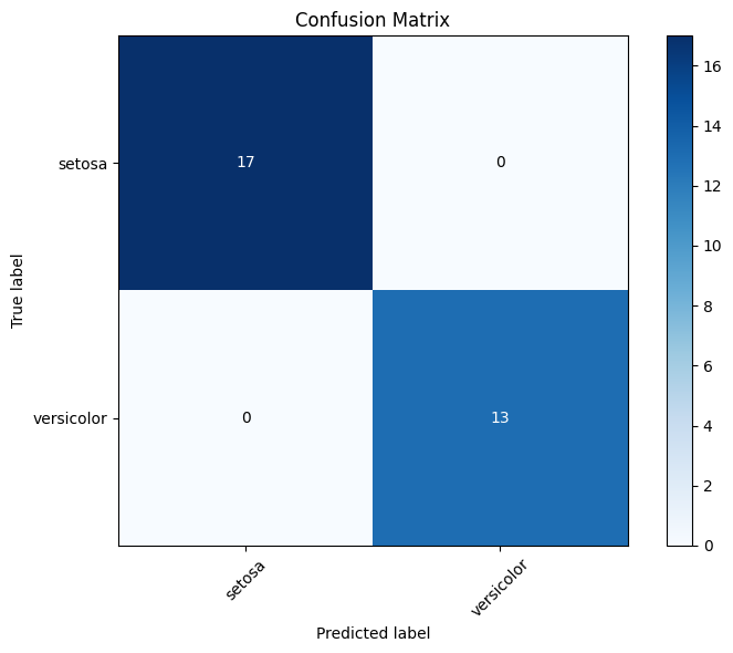

Instructions for Students:

Follow the steps to install the required libraries and load the dataset.
Train the logistic regression model and evaluate its performance.
Modify the code to use different datasets or add more features to the model.
Explore the impact of different hyperparameters on the model's performance.